Distributed Training at Scale

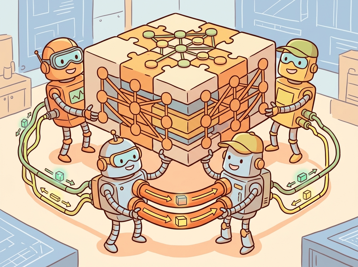
Training a large model on one GPU is like reading the entire internet through a keyhole. Distributed training lets you knock down the wall, provided all the GPUs agree on which wall and when.

Scale, Wall Demolishing AI Agent

6.6.1 Communication Primitives

Distributed training relies on collective communication operations to synchronize data between GPUs. Understanding these primitives is essential for reasoning about the communication overhead of different parallelism strategies.

These operations are implemented efficiently using ring or tree topologies. In a ring all-reduce with $P$ GPUs, each GPU sends and receives $2(P-1)/P$ times the tensor size, giving near-optimal bandwidth utilization regardless of the number of GPUs. The NCCL library (NVIDIA Collective Communications Library) provides highly optimized implementations for NVIDIA GPUs.

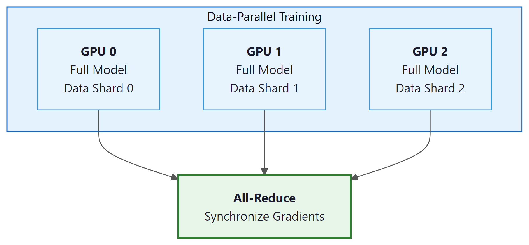
6.6.2 Data Parallelism (DDP)

Distributed Data Parallelism is the simplest and most widely used form of parallelism. Each GPU holds a complete copy of the model and processes a different subset of the training data. After each forward-backward pass, gradients are synchronized across all GPUs using all-reduce, ensuring that all copies perform identical parameter updates.

Figure 6.6.1a: In DDP, each GPU holds a full model copy and processes different data. Gradients are synchronized via all-reduce after each backward pass.

# DDP training with PyTorch
import torch
import torch.distributed as dist
from torch.nn.parallel import DistributedDataParallel as DDP
def setup_ddp(rank, world_size):
    dist.init_process_group("nccl", rank=rank, world_size=world_size)
    torch.cuda.set_device(rank)
def train_ddp(rank, world_size, model_class):
    setup_ddp(rank, world_size)
    # Each GPU gets a full model copy
    model = model_class().to(rank)
    model = DDP(model, device_ids=[rank])
    optimizer = torch.optim.AdamW(model.parameters(), lr=3e-4)
    for batch in dataloader:
        # Reset gradients from previous step
        optimizer.zero_grad()
        loss = model(batch)
        # Compute gradients via backpropagation
        loss.backward() # DDP auto-syncs gradients via all-reduce
        # Update weights using computed gradients
        optimizer.step()
        dist.destroy_process_group()

import torch
# FSDP training with PyTorch
from torch.distributed.fsdp import FullyShardedDataParallel as FSDP
from torch.distributed.fsdp import MixedPrecision, ShardingStrategy
# Mixed precision policy for FSDP
mp_policy = MixedPrecision(
    param_dtype=torch.bfloat16,
    reduce_dtype=torch.bfloat16,
    buffer_dtype=torch.bfloat16,
    )
# Wrap model with FSDP (full sharding = ZeRO Stage 3)
model = FSDP(
    model,
    sharding_strategy=ShardingStrategy.FULL_SHARD,
    mixed_precision=mp_policy,
    device_id=torch.cuda.current_device(),
    )
# Training loop is identical to standard PyTorch
for batch in dataloader:
    optimizer.zero_grad()
    loss = model(batch)
    loss.backward()
    optimizer.step()

6.6.3 Fully Sharded Data Parallelism (FSDP) and ZeRO

DDP's limitation is that every GPU must hold a complete copy of the model, gradients, and optimizer states. For a 7B model with AdamW, that is ~112 GB per GPU. FSDP (and the equivalent DeepSpeed ZeRO) resolves this by sharding these tensors across GPUs so each GPU stores only a fraction. These sharding techniques are equally important during fine-tuning of large models (see Section 16.4).

ZeRO Optimization Stages

• Stage 1: Shard optimizer states only. Each GPU stores 1/P of the optimizer states but keeps full parameters and gradients. Memory savings: ~4x reduction in optimizer memory.
• Stage 2: Shard optimizer states and gradients. After the backward pass, gradients are reduce-scattered so each GPU holds only its shard. Memory savings: further ~2x reduction.
• Stage 3: Shard everything (optimizer states, gradients, and parameters). Parameters are gathered on-demand for each layer's forward and backward pass, then discarded. Memory savings: total memory per GPU is 1/P of the full model state.

# FSDP (Fully Sharded Data Parallel) training with PyTorch.
# Each rank holds only 1/N of the parameters; missing shards are gathered
# just-in-time during forward/backward and freed immediately after.
import torch
import torch.distributed as dist
from torch.distributed.fsdp import (
    FullyShardedDataParallel as FSDP,
    MixedPrecision,
    ShardingStrategy,
)
from torch.distributed.fsdp.wrap import transformer_auto_wrap_policy
from functools import partial

# 1) Initialize the process group (one rank per GPU)
dist.init_process_group(backend="nccl")
local_rank = dist.get_rank()
torch.cuda.set_device(local_rank)

# 2) Build the model on each rank
from transformers import AutoModelForCausalLM
model = AutoModelForCausalLM.from_pretrained("meta-llama/Llama-3-8B")

# 3) Wrap with FSDP -- one wrapper per transformer block keeps memory low
from transformers.models.llama.modeling_llama import LlamaDecoderLayer
wrap_policy = partial(transformer_auto_wrap_policy, transformer_layer_cls={LlamaDecoderLayer})

model = FSDP(
    model,
    sharding_strategy=ShardingStrategy.FULL_SHARD,
    auto_wrap_policy=wrap_policy,
    mixed_precision=MixedPrecision(
        param_dtype=torch.bfloat16,
        reduce_dtype=torch.bfloat16,
        buffer_dtype=torch.bfloat16,
    ),
    device_id=torch.cuda.current_device(),
)

# 4) Normal-looking training step -- FSDP handles all-gather/reduce-scatter
optimizer = torch.optim.AdamW(model.parameters(), lr=3e-5)
for batch in train_loader:
    out = model(**batch)
    out.loss.backward()
    optimizer.step()
    optimizer.zero_grad(set_to_none=True)

dist.destroy_process_group()

6.6.4 Tensor Parallelism

Tensor parallelism splits individual layers across GPUs. For a linear layer $Y = XW$, the weight matrix $W$ can be split along its columns (column parallelism) or rows (row parallelism). Each GPU computes a portion of the output, and an all-reduce or all-gather combines the partial results.

Column Parallelism

Split $W$ into columns: $W = [W_{1} | W_{2}]$. GPU 0 computes $XW_{1}$, GPU 1 computes $XW_{2}$. The results are concatenated, requiring no communication in the forward pass (but an all-reduce in the backward pass). This is typically used for the first linear layer in the feed-forward network.

Row Parallelism

Split $W$ into rows. Each GPU processes a different slice of the input. The partial outputs are summed via all-reduce in the forward pass. This is typically used for the second linear layer in the feed-forward network.

In Megatron-LM style parallelism, column and row parallelism are combined so that the MLP block requires only one all-reduce in the forward pass and one in the backward pass. Tensor parallelism requires very fast interconnects (NVLink within a node) because communication happens at every layer. These same parallelism strategies are also essential for inference serving at scale, as discussed in Section 9.5.

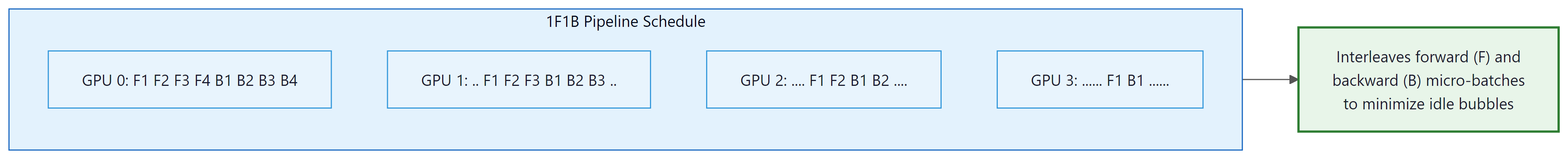
6.6.5 Pipeline Parallelism

Pipeline parallelism assigns different layers of the model to different GPUs. GPU 0 runs layers 0-15, GPU 1 runs layers 16-31, and so on. The input flows through the pipeline, with each GPU passing its output to the next.

The naive approach has a severe pipeline bubble problem: while GPU 0 is processing the forward pass, GPUs 1-3 are idle, and while GPU 3 is processing the backward pass, GPUs 0-2 are idle. The 1F1B (one forward, one backward) schedule mitigates this by splitting each batch into micro-batches and interleaving forward and backward passes across micro-batches. This keeps all GPUs active most of the time, though a small bubble remains at the beginning and end of each batch.

Figure 6.6.2a: The 1F1B pipeline schedule interleaves forward (F) and backward (B) micro-batches to minimize idle time (bubbles).