Mel Scale, Log-Mel Spectrograms, and MFCC

The raw STFT magnitude from Section G.2 is technically correct but perceptually wrong. Human hearing is roughly logarithmic in frequency: the gap between 100 Hz and 200 Hz feels musically equal to the gap between 1 kHz and 2 kHz, even though one is 100 Hz wide and the other is 1000 Hz wide. A linear spectrogram allocates one bin per 40 Hz everywhere, which wastes resolution at high frequencies (where humans cannot discriminate it) and starves low frequencies (where they can). The mel scale, the mel filter bank, and the log-mel spectrogram together fix this mismatch, and the result is the de facto input representation for nearly every speech and audio model. The illustration below makes the warping intuitive: imagine a piano whose bass keys are stretched wide and treble keys squeezed narrow, so each perceptual semitone takes equal physical space.

The Mel Scale

The mel scale maps physical frequency in hertz to a perceptual scale on which equal distances correspond to equal perceived pitch differences, calibrated by the Stevens, Volkmann, and Newman pitch experiments of 1937. The canonical (O'Shaughnessy) closed-form approximation is

with the inverse $f(m) = 700 \, (10^{m / 2595} - 1)$. The scale is approximately linear below 1 kHz and approximately logarithmic above it, mirroring the structure of the human cochlea. The exact constants differ slightly across the literature (HTK uses 2595, Slaney's formulation in librosa is slightly different); for practical audio ML the differences are imperceptible.

The Mel Filter Bank

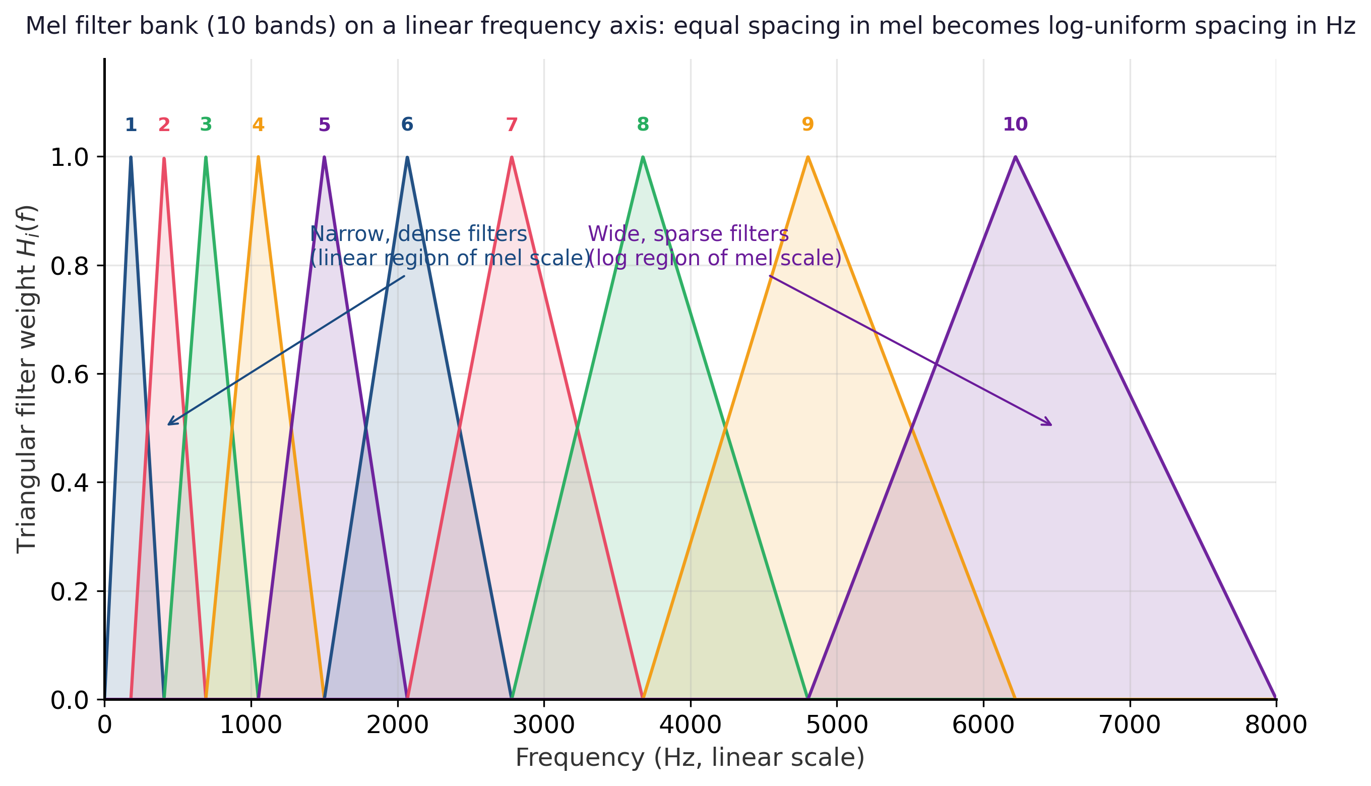
A mel filter bank is a set of $M$ triangular weighting functions (typically $M = 64$, $80$, or $128$) whose centers are spaced uniformly on the mel scale, hence approximately log-uniformly on the hertz scale above 1 kHz. Each triangle rises linearly from zero at its left edge to one at the center frequency of the next filter, then falls back to zero at the right edge; adjacent triangles overlap so that every STFT bin contributes to one or two filters. Concretely, if the $i$-th triangle has left, center, and right boundaries $f_{i-1}, f_i, f_{i+1}$ in hertz, the filter weight at FFT frequency $f$ is

The mel spectrogram is obtained by left-multiplying the power spectrogram $|X[m, k]|^2$ (of shape $T \times K$, where $K = N/2 + 1$) by the mel filter matrix $W \in \mathbb{R}^{M \times K}$, producing an $M \times T$ matrix in which row $i$ is the energy in the $i$-th mel band over time. Eighty mel bins is the standard for Whisper and most encoder-decoder ASR systems; 128 is common in music tagging. Figure G.3.1 overlays ten triangular filters on a linear-hertz axis to make the warping visible: the leftmost triangles are narrow and densely packed, while the rightmost ones spread out and overlap broadly, exactly the log-uniform spacing the mel scale prescribes.

Figure G.3.1: A mel filter bank with $M = 10$ triangular weighting functions plotted on a linear frequency axis. Equal spacing in mel-space (the spacing the centres were chosen at) appears as approximately linear spacing below 1 kHz and increasingly logarithmic spacing above it, giving low-frequency speech content far more resolution than high-frequency content.

The Log-Mel Spectrogram

One last step makes the representation neural-network-friendly. Acoustic energy spans many orders of magnitude (the dynamic range of speech is roughly 60 dB), and perception itself is logarithmic in intensity (a doubling of energy feels like a fixed increment in loudness, the basis of the decibel). The standard remedy is to take a log of the mel-filtered energies:

where $\varepsilon$ is a small floor (typically $10^{-6}$) that avoids $\log 0$ when a mel band is silent. The resulting log-mel spectrogram is the canonical input to Whisper, Wav2Vec 2.0, HuBERT, and most other modern speech models. It is conventionally followed by per-utterance or per-band mean-variance normalization to stabilize training.

import librosa
import numpy as np

# Load audio resampled to 16 kHz (the rate Whisper expects)
y, sr = librosa.load("speech.wav", sr=16000)

# Compute a log-mel spectrogram with Whisper-style parameters
mel = librosa.feature.melspectrogram(
    y=y,
    sr=sr,
    n_fft=400,          # 25 ms window at 16 kHz
    hop_length=160,     # 10 ms hop
    win_length=400,
    window="hann",
    n_mels=80,          # number of mel bands
    fmin=0.0,
    fmax=8000.0,        # Nyquist for 16 kHz
    power=2.0,          # power spectrogram, not amplitude
)

log_mel = np.log(mel + 1e-6)
print(log_mel.shape)    # (80, num_frames)

MFCC: The DCT of the Log-Mel

Before deep learning, classical ASR systems applied one more step: a discrete cosine transform (DCT) along the mel-band axis, producing mel-frequency cepstral coefficients (MFCC). The DCT decorrelates the mel bands (their values are highly correlated in natural speech) and concentrates energy into the first few coefficients, which is helpful for Gaussian-mixture acoustic models that assume diagonal covariance. The standard MFCC representation keeps the first 13 coefficients (sometimes augmented with first and second time differences, "delta" and "delta-delta" features), discarding the higher-order ones as noise.

For modern neural systems, the DCT is unnecessary: convolutions and self-attention learn whatever linear combinations of mel bands are useful, and the DCT throws away information that the network would otherwise have. The rule of thumb is therefore: use MFCC for classical GMM-HMM systems and for very small models where decorrelation helps; use log-mel for everything else, including all transformer-based ASR and audio generation models in Chapter 20.