PPO, RLHF Pipeline & the Full RL-to-LLM Alignment Picture

My value head said this state was great. My critic agreed. Then the environment quietly handed me a reward of zero and I had to update everyone's beliefs.

Reward, Slightly Disillusioned AI Agent

Having built up from rewards to advantages in Section 0.5, we now add the single ingredient that makes policy gradients safe enough to use on a giant LLM (PPO's clipped objective), then map everything we have learned onto how language models are actually aligned.

0.5.5 PPO: Stable Policy Updates

Proximal Policy Optimization (PPO) solves a critical problem with basic policy gradients: if a single update changes the policy too drastically, performance can collapse and never recover. PPO prevents this by clipping the update, ensuring each step is small and safe. For the full LLM-specific PPO loss including the KL penalty and the four-model PPO setup (policy, reference, reward, value), see the deep treatment in Section 18.1.3.

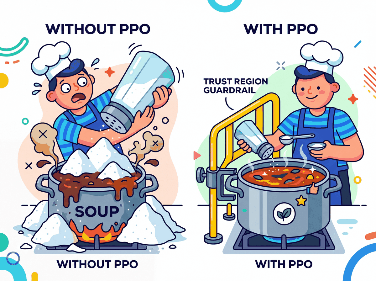
Here is the intuition. Imagine you are adjusting a recipe. You taste the soup, decide it needs more salt, and add some. With vanilla policy gradients, nothing stops you from dumping in the entire salt shaker. PPO is the rule that says: "Never add more than one pinch at a time." You can always taste again and add another pinch, but you cannot ruin the soup with a single reckless change.

Technically, PPO computes a ratio between the new policy's probability of an action and the old policy's probability. If this ratio drifts too far from 1.0 (typically beyond a range of 0.8 to 1.2), the gradient is clipped to zero. The policy still improves, but it cannot make a catastrophically large jump in a single step.

Formally, define the importance-sampling ratio between the new policy and the policy that collected the trajectory:

$$ r_t(\theta) = \frac{\pi_\theta(a_t \mid s_t)}{\pi_{\theta_{\text{old}}}(a_t \mid s_t)} $$

PPO maximizes the clipped surrogate objective, where $\hat{A}_t$ is the advantage estimate (typically GAE) and $\epsilon$ is the clip range (commonly 0.1 to 0.2):

$$ L^{\text{CLIP}}(\theta) = \mathbb{E}_t \Bigl[\, \min\bigl(r_t(\theta)\, \hat{A}_t,\; \mathrm{clip}(r_t(\theta), 1-\epsilon, 1+\epsilon)\, \hat{A}_t\bigr) \,\Bigr] $$

The $\min$ takes the more pessimistic of the unclipped and clipped objectives, so improving advantages above the clip range no longer pays. That single inequality is the entire safety mechanism.

# PPO clipped surrogate loss: the core update rule (Schulman et al., 2017).
# Inputs are tensors of new and old log-probabilities, the advantage estimate,
# and the value estimate; outputs the scalar loss to minimize.
import torch
import torch.nn.functional as F

def ppo_clip_loss(logp_new, logp_old, advantages, value_pred, value_target,
                  clip_eps: float = 0.2, vf_coef: float = 0.5, ent_coef: float = 0.01,
                  entropy=None):
    # Importance ratio r_t = pi_new / pi_old, computed in log-space for stability.
    ratio = torch.exp(logp_new - logp_old)

    # Unclipped and clipped surrogates; take the elementwise minimum.
    surr1 = ratio * advantages
    surr2 = torch.clamp(ratio, 1.0 - clip_eps, 1.0 + clip_eps) * advantages
    policy_loss = -torch.min(surr1, surr2).mean()  # negate: we maximize the surrogate

    # Value-function regression (MSE) and entropy bonus for exploration.
    value_loss = F.mse_loss(value_pred, value_target)
    ent_bonus  = entropy.mean() if entropy is not None else 0.0

    return policy_loss + vf_coef * value_loss - ent_coef * ent_bonus

0.5.6 From RL to LLM Training: The Complete Picture

We have built up the vocabulary piece by piece. Now let us assemble the full picture of how reinforcement learning powers LLM alignment. The mapping is direct and concrete:

Figure 0.5.5a: How RL concepts map to LLM training with RLHF. The LLM is the policy, tokens are actions, and the reward model provides the training signal.

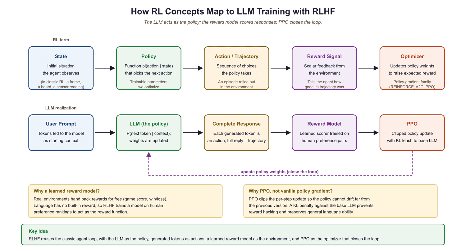
The RLHF training pipeline works as follows:

1. Supervised fine-tuning (SFT): First, the LLM is fine-tuned on high-quality human demonstrations. This gives the policy a good starting point.
2. Reward model training: Human annotators rank multiple model outputs for the same prompt. A separate neural network (the reward model) is trained to predict these human preferences.
3. RL optimization with PPO: The LLM generates responses to prompts. The reward model scores each response. PPO uses these scores to update the LLM's weights, nudging the probability distribution toward responses that score highly.

A critical detail: during the PPO phase, a KL (Kullback-Leibler) penalty prevents the RL-trained model from drifting too far from the SFT model. Without this constraint, the model might find degenerate responses that exploit the reward model (for example, generating repetitive flattery that scores highly but is useless). The KL penalty keeps the model close to its pretrained language abilities.

0.5.7 Putting It All Together: RL to LLM Alignment Pipeline

Let us trace the full journey from RL foundations to LLM training. An LLM begins as a pretrained model that can generate fluent text but may produce harmful, incorrect, or unhelpful responses. We want to steer it toward better behavior.

We frame this as an RL problem. The LLM is the agent (the policy). Each prompt starts a new episode. At each time step, the model picks a token (an action) based on its current context (the state). When the response is complete, the reward model assigns a score (the reward). PPO adjusts the model's weights so that high-scoring response patterns become more probable, while the clipping mechanism and KL penalty ensure the model does not lose its fluency or degenerate into reward hacking.

The dog analogy still holds at this scale. The dog does not understand English; it learns by trying actions and receiving treats. The LLM does not "understand" human values; it learns which outputs are valued by observing reward signals. The elegance of RL is that this simple loop of action, feedback, and adjustment can produce remarkably sophisticated behavior.

pip install matplotlib numpy

import matplotlib.pyplot as plt
import numpy as np
milestones = {
    1957: "Perceptron",
    1986: "Backpropagation",
    1997: "LSTM",
    2012: "AlexNet",
    2013: "Word2Vec",
    2014: "GANs",
    2017: "Transformer",
    2018: "BERT",
    2020: "GPT-3",
    2022: "InstructGPT\n(RLHF)",
    2023: "GPT-4",
    }
years = list(milestones.keys())
labels = list(milestones.values())
fig, ax = plt.subplots(figsize=(14, 3))
ax.scatter(years, [0] * len(years), s=80, zorder=5)
for i, (yr, lbl) in enumerate(zip(years, labels)):
    offset = 0.4 if i % 2 == 0 else -0.6
    ax.annotate(f"{lbl}\n({yr})", (yr, 0), (yr, offset),
        fontsize=8, ha="center", va="bottom" if offset > 0 else "top",
        arrowprops=dict(arrowstyle="-", color="gray", lw=0.8))
    ax.axhline(0, color="black", lw=0.8)
    ax.set_xlim(1955, 2025)
    ax.set_ylim(-1.2, 1.2)
    ax.axis("off")
    ax.set_title("Key ML and AI Milestones", fontsize=13, fontweight="bold")
    plt.tight_layout()
    plt.savefig("ml_timeline.png", dpi=150, bbox_inches="tight")
    plt.show()
    print("Timeline saved to ml_timeline.png")

import numpy as np
class GridWorld:
    def __init__(self, size=4):
        self.size = size
        self.state = (0, 0)
        self.goal = (size - 1, size - 1)
        self.actions = [(0, 1), (0, -1), (1, 0), (-1, 0)] # right, left, down, up
    def reset(self):
        self.state = (0, 0)
        return self.state
    def step(self, action_idx):
        dr, dc = self.actions[action_idx]
        r = max(0, min(self.size - 1, self.state[0] + dr))
        c = max(0, min(self.size - 1, self.state[1] + dc))
        self.state = (r, c)
        done = self.state == self.goal
        reward = 1.0 if done else -0.01
        return self.state, reward, done
env = GridWorld()
print(f"Start: {env.reset()}, Goal: {env.goal}")

Q = np.zeros((4, 4, 4)) # states (4x4) x actions (4)
alpha, gamma, epsilon = 0.1, 0.99, 0.1
episodes = 500
for ep in range(episodes):
state = env.reset()
for _ in range(100): # max steps
# Epsilon-greedy action selection
if np.random.random() < epsilon:
action = np.random.randint(4)
else:
action = np.argmax(Q[state[0], state[1]])
next_state, reward, done = env.step(action)
# Q-learning update
best_next = np.max(Q[next_state[0], next_state[1]])
Q[state[0], state[1], action] += alpha * (
reward + gamma * best_next - Q[state[0], state[1], action]
)
state = next_state
if done:
break
# Show learned policy
action_names = ["right", "left", "down", "up"]
print("Learned policy:")
for r in range(4):
row = []
for c in range(4):
row.append(action_names[np.argmax(Q[r, c])])
print(f" Row {r}: {row}")

import numpy as np
import matplotlib.pyplot as plt
v = np.max(Q, axis=2) # Value function: max Q at each state
fig, ax = plt.subplots(figsize=(5, 5))
im = ax.imshow(v, cmap="YlOrRd", interpolation="nearest")
for r in range(4):
    for c in range(4):
        ax.text(c, r, f"{v[r, c]:.2f}", ha="center", va="center", fontsize=11)
        ax.set_title("Learned Value Function V(s) = max Q(s,a)")
        ax.set_xlabel("Column")
        ax.set_ylabel("Row")
        plt.colorbar(im, ax=ax, shrink=0.8)
        plt.tight_layout()
        plt.savefig("gridworld_values.png", dpi=150)
        plt.show()