Distributed Training at Scale

Training a large model on one GPU is like reading the entire internet through a keyhole. Distributed training lets you knock down the wall, provided all the GPUs agree on which wall and when.

Scale, Wall Demolishing AI Agent

1. Communication Primitives

Distributed training relies on collective communication operations to synchronize data between GPUs. Understanding these primitives is essential for reasoning about the communication overhead of different parallelism strategies.

These operations are implemented efficiently using ring or tree topologies. In a ring all-reduce with $P$ GPUs, each GPU sends and receives $2(P-1)/P$ times the tensor size, giving near-optimal bandwidth utilization regardless of the number of GPUs. The NCCL library (NVIDIA Collective Communications Library) provides highly optimized implementations for NVIDIA GPUs.

2. Data Parallelism (DDP)

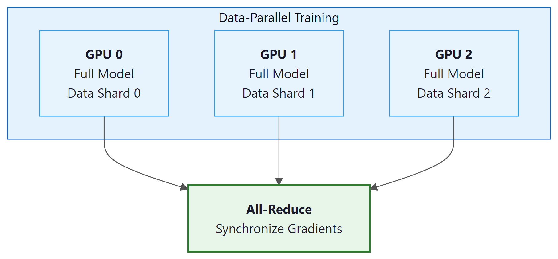
Distributed Data Parallelism is the simplest and most widely used form of parallelism. Each GPU holds a complete copy of the model and processes a different subset of the training data. After each forward-backward pass, gradients are synchronized across all GPUs using all-reduce, ensuring that all copies perform identical parameter updates. Code Fragment 6.6.1 below puts this into practice.

Figure 6.6.3: In DDP, each GPU holds a full model copy and processes different data. Gradients are synchronized via all-reduce after each backward pass.

# DDP training with PyTorch
import torch
import torch.distributed as dist
from torch.nn.parallel import DistributedDataParallel as DDP

def setup_ddp(rank, world_size):
    dist.init_process_group("nccl", rank=rank, world_size=world_size)
    torch.cuda.set_device(rank)

def train_ddp(rank, world_size, model_class):
    setup_ddp(rank, world_size)

    # Each GPU gets a full model copy
    model = model_class().to(rank)
    model = DDP(model, device_ids=[rank])

    optimizer = torch.optim.AdamW(model.parameters(), lr=3e-4)

    for batch in dataloader:
        # Reset gradients from previous step
        optimizer.zero_grad()
        loss = model(batch)
        # Compute gradients via backpropagation
        loss.backward()     # DDP auto-syncs gradients via all-reduce
        # Update weights using computed gradients
        optimizer.step()

    dist.destroy_process_group()

# FSDP training with PyTorch
from torch.distributed.fsdp import FullyShardedDataParallel as FSDP
from torch.distributed.fsdp import MixedPrecision, ShardingStrategy

# Mixed precision policy for FSDP
mp_policy = MixedPrecision(
    param_dtype=torch.bfloat16,
    reduce_dtype=torch.bfloat16,
    buffer_dtype=torch.bfloat16,
)

# Wrap model with FSDP (full sharding = ZeRO Stage 3)
model = FSDP(
    model,
    sharding_strategy=ShardingStrategy.FULL_SHARD,
    mixed_precision=mp_policy,
    device_id=torch.cuda.current_device(),
)

# Training loop is identical to standard PyTorch
for batch in dataloader:
    optimizer.zero_grad()
    loss = model(batch)
    loss.backward()
    optimizer.step()

3. Fully Sharded Data Parallelism (FSDP) and ZeRO

DDP's limitation is that every GPU must hold a complete copy of the model, gradients, and optimizer states. For a 7B model with AdamW, that is ~112 GB per GPU. FSDP (and the equivalent DeepSpeed ZeRO) resolves this by sharding these tensors across GPUs so each GPU stores only a fraction. These sharding techniques are equally important during fine-tuning of large models (see Section 13.4).

ZeRO Optimization Stages

• Stage 1: Shard optimizer states only. Each GPU stores 1/P of the optimizer states but keeps full parameters and gradients. Memory savings: ~4x reduction in optimizer memory.
• Stage 2: Shard optimizer states and gradients. After the backward pass, gradients are reduce-scattered so each GPU holds only its shard. Memory savings: further ~2x reduction.
• Stage 3: Shard everything (optimizer states, gradients, and parameters). Parameters are gathered on-demand for each layer's forward and backward pass, then discarded. Memory savings: total memory per GPU is 1/P of the full model state.

4. Tensor Parallelism

Tensor parallelism splits individual layers across GPUs. For a linear layer $Y = XW$, the weight matrix $W$ can be split along its columns (column parallelism) or rows (row parallelism). Each GPU computes a portion of the output, and an all-reduce or all-gather combines the partial results.

Column Parallelism

Split $W$ into columns: $W = [W_{1} | W_{2}]$. GPU 0 computes $XW_{1}$, GPU 1 computes $XW_{2}$. The results are concatenated, requiring no communication in the forward pass (but an all-reduce in the backward pass). This is typically used for the first linear layer in the feed-forward network.

Row Parallelism

Split $W$ into rows. Each GPU processes a different slice of the input. The partial outputs are summed via all-reduce in the forward pass. This is typically used for the second linear layer in the feed-forward network.

In Megatron-LM style parallelism, column and row parallelism are combined so that the MLP block requires only one all-reduce in the forward pass and one in the backward pass. Tensor parallelism requires very fast interconnects (NVLink within a node) because communication happens at every layer. These same parallelism strategies are also essential for inference serving at scale, as discussed in Section 8.4.

5. Pipeline Parallelism

Pipeline parallelism assigns different layers of the model to different GPUs. GPU 0 runs layers 0-15, GPU 1 runs layers 16-31, and so on. The input flows through the pipeline, with each GPU passing its output to the next.

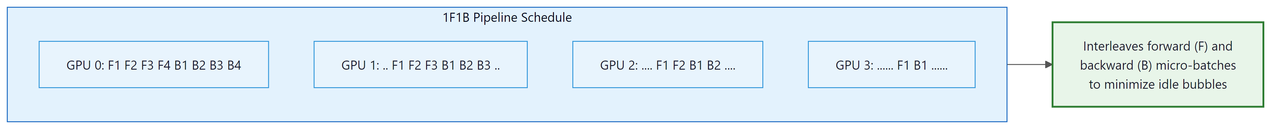
The naive approach has a severe pipeline bubble problem: while GPU 0 is processing the forward pass, GPUs 1-3 are idle, and while GPU 3 is processing the backward pass, GPUs 0-2 are idle. The 1F1B (one forward, one backward) schedule mitigates this by splitting each batch into micro-batches and interleaving forward and backward passes across micro-batches. This keeps all GPUs active most of the time, though a small bubble remains at the beginning and end of each batch.

Figure 6.6.4: The 1F1B pipeline schedule interleaves forward (F) and backward (B) micro-batches to minimize idle time (bubbles).

6. Mixed Precision Training

Mixed precision reduces memory usage and increases throughput by using lower-precision number formats for most computations while keeping critical accumulations in higher precision.

FP8 Training at Scale

DeepSeek V3 (covered in Section 7.2) demonstrated successful FP8 mixed-precision training at 671B parameters, the first large-scale demonstration of FP8 for LLM pre-training. The approach uses E4M3 format for forward pass activations (more precision, narrower range) and E5M2 for gradients (wider range, less precision). Per-tensor dynamic scaling factors are maintained to prevent overflow and underflow. FP8 training provides roughly 2x memory reduction and higher throughput compared to BF16 with minimal quality degradation.

7. Gradient Checkpointing

During the backward pass, computing gradients requires the activations from the forward pass. Normally all activations are stored in memory, consuming enormous amounts of GPU memory (proportional to batch size, sequence length, and hidden dimension). Gradient checkpointing (also called activation checkpointing) saves memory by storing only a subset of activations and recomputing the rest during the backward pass. The tradeoff is approximately 33% additional compute in exchange for a large reduction in activation memory. Code Fragment 6.6.3 below puts this into practice.

# Gradient checkpointing in PyTorch
from torch.utils.checkpoint import checkpoint

class CheckpointedTransformer(nn.Module):
    def __init__(self, layers):
        super().__init__()
        self.layers = nn.ModuleList(layers)

    def forward(self, x):
        for layer in self.layers:
            # Recompute activations during backward instead of storing
            x = checkpoint(layer, x, use_reentrant=False)
        return x

# Memory comparison
seq_len, hidden, num_layers, batch = 2048, 4096, 32, 8
bytes_per_elem = 2  # BF16

# Without checkpointing: store all layer activations
no_ckpt = batch * seq_len * hidden * num_layers * bytes_per_elem
# With checkpointing: store only input to each checkpointed segment
with_ckpt = batch * seq_len * hidden * 1 * bytes_per_elem  # only 1 activation

print(f"Activation memory without checkpointing: {no_ckpt / 1e9:.1f} GB")
print(f"Activation memory with checkpointing:    {with_ckpt / 1e9:.2f} GB")
print(f"Memory saved: {(1 - with_ckpt/no_ckpt)*100:.0f}%")

Expert Parallelism for MoE Training

Mixture-of-Experts models introduce a parallelism dimension that dense models do not have: expert parallelism. In an MoE layer, each token is routed to a small subset of experts (typically 1 or 2 out of dozens or hundreds). Expert parallelism distributes the experts themselves across GPUs, so that each GPU hosts a different subset of the expert FFN blocks. When a token is routed to an expert that lives on another GPU, an all-to-all communication operation transfers the token's hidden state to the appropriate device, and the result is sent back after computation.

The communication pattern differs fundamentally from tensor parallelism. In tensor parallelism, every GPU participates in computing every token (splitting the matrix multiply). In expert parallelism, each GPU only computes the tokens routed to its local experts. This means the amount of computation per GPU varies depending on how the router distributes tokens, making load balancing critically important. If one expert receives disproportionately many tokens, the GPU hosting that expert becomes the bottleneck while others sit idle.

DeepSeek-V3 provides a detailed case study. With 256 routed experts and 1 shared expert, the experts are distributed across GPUs such that each GPU hosts a manageable subset. DeepSeek-V3 uses an auxiliary-loss-free load balancing mechanism with a per-expert bias term that the system adjusts dynamically during training to maintain even expert utilization. This avoids the traditional auxiliary loss approach, which adds a balancing penalty to the training objective and can distort the learning signal. The all-to-all communication is overlapped with computation by pipelining the expert dispatch: while one micro-batch's tokens are being routed and computed on remote experts, the next micro-batch's routing decisions are already being made.

In practice, expert parallelism is combined with the other strategies. A typical configuration for training a large MoE model on 256 GPUs might use tensor parallelism of 8 within each node, expert parallelism of 8 across nodes within a pod, and data parallelism of 4 across pods. The key constraint is that expert parallelism requires all-to-all communication, which has higher latency than the all-reduce used in data parallelism. Placing expert parallelism on a network tier with sufficient bandwidth (typically InfiniBand HDR or better) is essential. As models scale to hundreds or thousands of experts, expert parallelism has become the fourth essential dimension of the "4D parallelism" strategy used in modern large-scale training.

8. Combining Parallelism Strategies

Real-world large-scale training combines multiple parallelism strategies in a hierarchy. A common configuration for training a 70B model on 512 GPUs might use tensor parallelism with degree 8 within each node (leveraging fast NVLink), pipeline parallelism with degree 8 across nodes, and data parallelism with degree 8 across pipeline-parallel groups. This 3D parallelism approach matches each strategy to the communication bandwidth available at each level of the hardware hierarchy.

The parallelism strategies above partition the model across devices, but they all assume the input sequence fits in a single GPU's memory. As context windows grow to 128K tokens and beyond, the attention matrix itself becomes the bottleneck. This requires parallelizing along a new dimension: the sequence itself.

9. Ring Attention and Sequence Parallelism for Long-Context Training

The push toward million-token context windows has made sequence-dimension parallelism a critical fourth axis of distributed training, alongside data, tensor, and pipeline parallelism. Standard self-attention requires materializing an attention matrix of size $L \times L$ (where $L$ is the sequence length), which grows quadratically. For a 128K-token sequence, this matrix alone would require over 60 GB of memory in FP32, exceeding the capacity of any single GPU. Sequence parallelism and ring attention solve this by distributing the sequence dimension across multiple devices.

Sequence Parallelism: Splitting the Sequence

Sequence parallelism partitions each input sequence into contiguous chunks, assigning each chunk to a different GPU. For non-attention operations (feed-forward layers, normalization, embedding lookups), this is straightforward because these operations process each token independently. The challenge arises with self-attention, where every token must attend to every other token. Naive partitioning would require each GPU to receive the full key-value (KV) pairs from all other GPUs at every attention layer, introducing prohibitive communication overhead. Megatron-LM's sequence parallelism (Korthikanti et al., 2022) addressed this for the non-attention components of transformer layers, splitting LayerNorm and dropout operations along the sequence dimension. This alone saves significant activation memory, as dropout masks and normalization statistics scale linearly with sequence length.

Ring Attention: Communication-Efficient Long Context

Ring Attention (Liu et al., 2023) provides an elegant solution for distributing the attention computation itself. The core idea is to arrange GPUs in a logical ring and overlap attention computation with communication. Each GPU holds a chunk of the query (Q) tokens permanently and receives key-value (KV) chunks from its neighbors in a round-robin fashion. The algorithm proceeds in $P$ steps (where $P$ is the number of GPUs in the ring):

1. Each GPU computes attention between its local Q chunk and its local KV chunk.
2. While computing, each GPU asynchronously sends its KV chunk to the next GPU in the ring and receives a KV chunk from the previous GPU.
3. In the next step, each GPU computes attention between its local Q and the newly received KV chunk.
4. After $P$ steps, every Q chunk has attended to every KV chunk, and the attention output is complete.

The key insight is that the communication of KV chunks is overlapped with the computation of attention, hiding the communication latency behind the compute. With modern interconnects (NVLink at 900 GB/s on H100, InfiniBand at 400 Gb/s), the communication can be fully hidden as long as the per-chunk compute time exceeds the transfer time. In practice, this holds for chunks of 4K tokens or larger on H100 GPUs. The memory per GPU is reduced from $O(L^{2})$ to $O(L^{2}/P)$ for the attention matrix, and $O(L/P)$ for KV storage, enabling linear memory scaling with the number of ring participants.

Striped Attention and Hybrid Approaches

A limitation of basic ring attention is load imbalance when using causal (autoregressive) attention masks. Because causal attention is triangular (token $i$ attends only to tokens $1$ through $i$), GPUs holding later chunks do more work than those holding earlier chunks. Striped Attention (Brandon et al., 2023) addresses this by distributing tokens in an interleaved (striped) pattern rather than contiguous blocks: GPU 0 gets tokens 0, P, 2P, ...; GPU 1 gets tokens 1, P+1, 2P+1, ...; and so on. This ensures each GPU processes roughly equal amounts of causal attention work, improving utilization from approximately 50% (for contiguous chunking with causal masks) to near 100%.

Meta's Llama 3 training (2024) used a hybrid approach that combined ring attention (called "context parallelism" in their terminology) with tensor parallelism and data parallelism for training on sequences up to 128K tokens. Their implementation placed the ring attention ring within a single node's 8 GPUs (leveraging NVLink bandwidth), while using tensor parallelism across nodes and data parallelism across node groups. This hierarchical design matches communication intensity to available bandwidth at each level. DeepSeek-V2 and Qwen 2.5 employed similar strategies for their long-context training phases.

# pip install accelerate
from accelerate import Accelerator

accelerator = Accelerator(mixed_precision="bf16")

# Wrap model, optimizer, and dataloader in one call
model, optimizer, dataloader = accelerator.prepare(
    model, optimizer, dataloader
)

for batch in dataloader:
    outputs = model(**batch)
    loss = outputs.loss
    accelerator.backward(loss)
    optimizer.step()
    optimizer.zero_grad()

# Launch with: accelerate launch --num_processes 4 train.py

# pip install deepspeed
# deepspeed_config.json:
# {
#   "bf16": {"enabled": true},
#   "zero_optimization": {"stage": 3, "offload_param": {"device": "cpu"}},
#   "train_batch_size": 32,
#   "gradient_accumulation_steps": 4
# }

# Launch training:
# deepspeed train.py --deepspeed deepspeed_config.json

# Or use with HuggingFace Accelerate:
# accelerate launch --use_deepspeed \
#     --deepspeed_config_file deepspeed_config.json train.py

Practical Considerations

When implementing sequence parallelism for long-context training, several practical considerations apply. First, ring attention typically requires that the sequence length is evenly divisible by the ring size; padding shorter sequences wastes compute proportionally. Second, position encodings (particularly RoPE) must be consistent across the distributed sequence: each GPU must use the correct positional indices for its assigned tokens, not indices starting from zero. Third, the gradients for attention computations across the ring require careful accumulation during the backward pass, as each partial attention result must be combined with the correct log-sum-exp normalization factors to produce numerically stable softmax gradients. Frameworks like Megatron-LM and DeepSpeed-Ulysses provide production-ready implementations of these techniques, while the Llama 3 training code release includes Meta's context parallelism implementation for reference.