"A spectrogram is to a waveform what a printed score is to a performance: most of the information, almost none of the storage, exactly the right view for the next step in the pipeline."
Echo, Pitch-Perfect AI Agent
Every audio model in this chapter consumes one of three input formats: a raw waveform tensor, a complex-valued short-time Fourier transform (STFT), or a log-mel spectrogram. This section installs the signal-processing vocabulary needed to move between those formats, the decibel scale used everywhere in audio plots, and the HuggingFace datasets workflow that resamples, preprocesses, and batches audio into model-ready tensors. The payoff is that the rest of the chapter can say "Whisper consumes an 80-bin log-mel spectrogram at 100 Hz" without leaving the reader guessing what any of those numbers mean.
Why this lives in an LLM and Agents book. Every audio LLM and conversational agent in later chapters (Whisper, Bark, AudioLM, MusicGen, Moshi, and the speech leg of every voice agent) consumes log-mel spectrograms or codec tokens that begin life as the signal-processing primitives in this section. Without the right sampling rate, frame length, and feature dimension the transformer either hallucinates or refuses; the audio front-end is the silent prerequisite for every multimodal LLM that ships voice.
Prerequisites
This section assumes the reader has seen a transformer (Chapter 3) and the HuggingFace pipeline abstraction (Chapter 7). Comfort with numpy arrays, simple complex numbers, and basic trigonometry is enough. Deeper signal-processing background (the Nyquist-Shannon theorem, the convolution theorem, the DCT derivation) lives in Appendix G: Signal Processing for Audio. No prior audio engineering experience is required.
20.0.1.1 Waveforms, Sampling Rate, and Bit Depth
A sound is a pressure variation in air. A microphone converts that variation into a continuous voltage $S(t)$ and an analog-to-digital converter samples it at uniform intervals to produce a discrete sequence $S_i = S(i / f_s)$ where $f_s$ is the sampling rate in samples per second (hertz, Hz). The standard sampling rates in audio AI are 16 kHz for speech (Whisper, wav2vec 2.0, HuBERT all expect 16 kHz input), 24 kHz for high-quality speech and EnCodec defaults, 44.1 kHz for CD audio, and 48 kHz for professional music. The Nyquist theorem says a sampling rate of $f_s$ can faithfully represent frequencies up to $f_s / 2$, so 16 kHz audio captures content up to 8 kHz, which covers all speech information but loses the highest musical overtones.
Bit depth measures how many bits encode each sample's amplitude. The standard formats are 16-bit signed integers (CD audio, most speech datasets), 24-bit (professional music), and 32-bit floats (intermediate processing). A 16-bit sample has 65,536 possible amplitude values, giving a theoretical dynamic range of about 96 dB, which is well above the noise floor of any normal recording environment.
The number that matters when budgeting transformer context is the length of the resulting tensor. A 30-second clip at 16 kHz is 480,000 samples. Feeding that directly to a transformer is impossible (the attention cost is quadratic in sequence length), which is why every modern audio model first downsamples through a convolutional front-end or converts to a spectrogram. The log-mel spectrograms that Whisper consumes are roughly 3,000 frames long for a 30-second clip, a 160x compression, and even that uses two convolutional layers in the encoder to halve the length further before the transformer blocks see it.
The single most common audio-AI bug is feeding 44.1 kHz audio to a model trained on 16 kHz. The model will not error; it will just transcribe gibberish, because the spectrogram the model sees corresponds to a sound played at 2.76x the original speed. Always call librosa.resample or torchaudio.functional.resample (or use HuggingFace datasets.cast_column("audio", Audio(sampling_rate=16_000))) before inference. Whisper's HuggingFace processor will print a warning but does not refuse; many other processors do neither.
Steps
import librosa
import librosa.display
import matplotlib.pyplot as plt

# librosa ships with several example clips; "trumpet" is a clean 6-second tone
y, sr = librosa.load(librosa.ex("trumpet"))
print(f"Loaded {len(y)} samples at {sr} Hz")  # 132300 samples at 22050 Hz
print(f"Duration: {len(y) / sr:.2f} seconds")  # 6.00 seconds

# librosa.load defaults to mono and resamples to 22050 Hz. Override either:
y16, sr16 = librosa.load(librosa.ex("trumpet"), sr=16_000, mono=True)

fig, ax = plt.subplots(figsize=(8, 2.5))
librosa.display.waveshow(y16, sr=sr16, ax=ax)
ax.set(title="Trumpet waveform (16 kHz mono)", xlabel="Time (s)", ylabel="Amplitude")
plt.tight_layout()librosa.ex(name) helper resolves a curated set of public-domain clips ("trumpet", "fishin", "brahms", "choice") to local cached paths. The default sample rate of 22.05 kHz comes from librosa's history with music research; speech work usually overrides to sr=16_000. librosa.display.waveshow uses a peak envelope renderer that stays readable even at minute-scale durations.20.0.1.2 The Frequency Domain: From FFT to STFT
The time-domain waveform $S_i$ is not what a transformer wants to look at, because speech and music structure live in the frequency distribution of energy, not in individual samples. A pure tone of frequency $f_0$ and amplitude $A$ is $A \sin(2\pi f_0 t - \phi)$; its frequency spectrum is a single spike at $f_0$. A real-world sound is a superposition of many such tones, and the Fourier transform decomposes the waveform into its frequency components.
For discrete signals, the Discrete Fourier Transform (DFT) of an $N$-sample window computes the complex amplitudes at $N$ equally spaced frequencies:
The Fast Fourier Transform (FFT) algorithm computes the DFT in $O(N \log N)$ time, and is the workhorse behind every spectrogram in this book. Because audio is real-valued, the negative-frequency half of $X_k$ is the conjugate of the positive half, so libraries expose a "real" FFT (numpy's np.fft.rfft) that returns only the $N/2 + 1$ non-redundant bins.
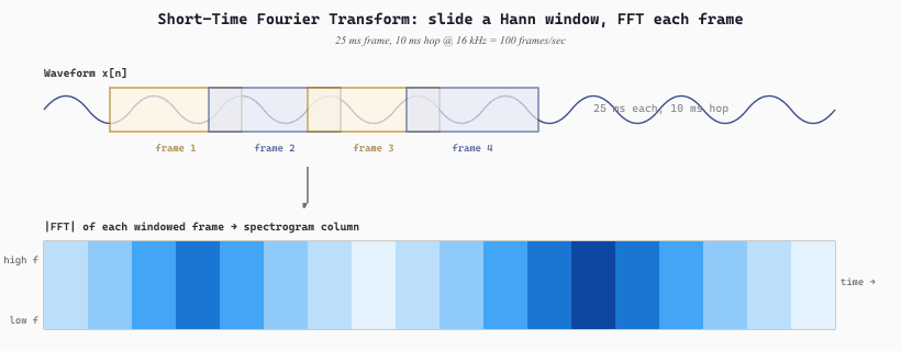
A single FFT over an entire utterance throws away time information: it tells the reader which frequencies are present somewhere in the clip, but not when. The Short-Time Fourier Transform (STFT) fixes this by sliding a short window along the signal and applying an FFT to each window. The standard conventions for speech at 16 kHz are a 25 ms frame length (400 samples) and a 10 ms hop length (160 samples), giving 100 frames per second of audio. A 30-second clip then becomes a 3000-frame STFT, which is exactly the input shape Whisper expects.
Before applying the FFT to each window, the signal must be multiplied by a tapered window function to suppress the discontinuity at the window edges that would otherwise smear energy across all frequencies (spectral leakage). The two standard windows are the Hann window $w_n = 0.5 (1 - \cos(2\pi n / (N-1)))$ and the Hamming window $w_n = 0.54 - 0.46 \cos(2\pi n / (N-1))$, both raised cosines that taper smoothly to zero at the edges.
(n_fft / 2 + 1, n_frames): rows are frequency bins, columns are time frames, and the value at $(k, t)$ is the energy at frequency $k$ in time frame $t$.20.0.1.3 The Decibel Scale
Sound intensity spans an enormous dynamic range. The threshold of human hearing is about $10^{-12}$ W/m^2; a jet engine at takeoff is about $10^2$ W/m^2, a factor of $10^{14}$ apart. Plotting any spectrum on a linear amplitude axis throws away nearly all the visible detail in the low-amplitude regions. The decibel (dB) is the logarithmic scale that fixes this:
On this scale silence is 0 dB, a quiet room is around 30 dB, normal conversation about 60 dB, a busy street 80 dB, a rock concert 110 to 120 dB, and a jet engine at 10 m about 130 dB. Audio plots almost always use dB on the amplitude axis because perception itself is approximately logarithmic: a 10 dB increase sounds roughly twice as loud, regardless of the starting point.
In practice librosa exposes two conversion helpers. librosa.amplitude_to_db(np.abs(D)) converts a complex STFT $D$ to dB, treating the input as amplitude (so it uses $20 \log_{10}|D|$). librosa.power_to_db(S) takes a power spectrum (the squared magnitude) and uses $10 \log_{10} S$. Both clip very small values to a floor (default 80 dB below the maximum) to keep plots readable.
Steps
import librosa
import librosa.display
import matplotlib.pyplot as plt
import numpy as np

y, sr = librosa.load(librosa.ex("trumpet"), sr=22_050)

# A single FFT of the first 4096 samples shows the harmonic spectrum.
window = np.hanning(4096)
spectrum = np.fft.rfft(y[:4096] * window)
spectrum_db = librosa.amplitude_to_db(np.abs(spectrum), ref=np.max)
freqs = np.fft.rfftfreq(4096, d=1 / sr)

fig, axes = plt.subplots(1, 2, figsize=(12, 3.5))
axes[0].semilogx(freqs, spectrum_db)
axes[0].set(title="Single-frame spectrum (Hanning-windowed)",
            xlabel="Frequency (Hz)", ylabel="Amplitude (dB)",
            xlim=(10, sr / 2))

# A full STFT shows how the harmonic structure evolves over time.
D = librosa.stft(y, n_fft=2048, hop_length=512)
D_db = librosa.amplitude_to_db(np.abs(D), ref=np.max)
img = librosa.display.specshow(D_db, sr=sr, hop_length=512,
                                x_axis="time", y_axis="hz", ax=axes[1])
axes[1].set(title="STFT spectrogram (linear-frequency, dB amplitude)")
fig.colorbar(img, ax=axes[1], format="%+2.0f dB")
plt.tight_layout()ref=np.max argument normalizes the dB scale so the peak is at 0 dB, a convention that lets readers compare spectrograms across clips of different absolute loudness.20.0.1.4 The Mel Scale and the Log-Mel Spectrogram
Human hearing is not linear in frequency. A trained ear can easily distinguish 500 Hz from 1000 Hz, but the same 500 Hz gap between 5000 Hz and 5500 Hz is barely perceptible. Stevens, Volkmann, and Newman quantified this in 1937 with the mel scale, which warps frequency so that equal mel intervals correspond to equal perceived pitch differences. The standard formula is:
where $f$ is in hertz and $m$ is in mels. Below about 500 Hz the mel scale is nearly linear in $f$; above that it becomes increasingly logarithmic, so the upper octaves are compressed.
A mel filterbank implements this warp by summing the STFT magnitudes into a smaller set of overlapping triangular filters spaced uniformly on the mel axis. The standard size for speech is 80 filters covering 0 to 8 kHz (Whisper, AST, wav2vec 2.0 all use 80-bin mel). The filters are denser at low frequencies where pitch discrimination matters most and broader at high frequencies where it does not.
Applying the mel filterbank to a power-magnitude STFT yields a mel spectrogram; taking the log of that yields the log-mel spectrogram, the canonical input format for modern speech and audio models:
where $M_{m,k}$ is the mel filterbank matrix (one row per mel bin, one column per linear frequency bin) and $\epsilon$ is a small constant (typically $10^{-10}$) to avoid taking $\log 0$. The log compression mirrors the decibel scale: it makes the network's input distribution more symmetric and helps gradient flow.
Whisper's input tensor shape (3000, 80) decomposes exactly as the STFT plus mel filterbank pipeline above. A 30-second clip at 16 kHz with a 25 ms frame and 10 ms hop produces $30 \times 100 = 3000$ frames. The 80 comes from 80 mel filterbank bins covering 0 to 8 kHz. Every "Whisper expects log-mel" claim in the chapter reduces to running librosa.feature.melspectrogram(y, sr=16000, n_fft=400, hop_length=160, n_mels=80) followed by librosa.power_to_db. AST uses the same (3000, 80) shape for 30-second clips. The pretrained model is locked to these dimensions, which is why a feature extractor is a non-optional part of every audio pipeline.
Steps
import librosa
import librosa.display
import numpy as np
import matplotlib.pyplot as plt

y, sr = librosa.load(librosa.ex("trumpet"), sr=16_000)

# Compute the mel spectrogram on a power scale, then convert to dB.
S = librosa.feature.melspectrogram(
    y=y, sr=sr,
    n_fft=400,        # 25 ms frame at 16 kHz
    hop_length=160,   # 10 ms hop
    n_mels=80,        # the canonical Whisper / AST setting
    fmin=0, fmax=8000,
)
S_db = librosa.power_to_db(S, ref=np.max)

print(S_db.shape)  # (80, n_frames); each frame is 10 ms

fig, ax = plt.subplots(figsize=(8, 3))
img = librosa.display.specshow(S_db, sr=sr, hop_length=160,
                                x_axis="time", y_axis="mel",
                                fmin=0, fmax=8000, ax=ax)
ax.set(title="80-bin log-mel spectrogram (Whisper / AST input format)")
fig.colorbar(img, ax=ax, format="%+2.0f dB")
plt.tight_layout()S_db is the exact tensor Whisper's feature extractor produces internally (modulo a fixed normalization step), and any model with "log-mel input" in its model card consumes this format. Reader who wants the precise Whisper preprocessing should use transformers.WhisperFeatureExtractor instead; reader who wants to feed an arbitrary 80-bin log-mel into a custom model should start from this snippet.20.0.1.5 MFCCs: The Classical Front-End
Mel-Frequency Cepstral Coefficients (MFCCs) were the dominant audio feature from the 1980s through the deep-learning revolution around 2014. The pipeline is one step longer than log-mel: take the log-mel spectrogram, then apply a Discrete Cosine Transform (DCT) along the mel axis and keep only the first $K$ coefficients (typically $K = 13$, sometimes augmented with first and second time derivatives for 39 total features per frame).
The DCT serves two purposes. First, it decorrelates the mel bins, which was important for classical Gaussian mixture model (GMM) classifiers that assumed diagonal covariance. Second, it concentrates information in the low-order coefficients, so dropping all but the first 13 removes high-order detail that classical models could not exploit anyway. The result is a compact 13-dimensional feature vector per frame, an enormous compression over the 80-bin log-mel.
Modern deep models do not use MFCCs. The decorrelation and dimensionality reduction that MFCCs provide are exactly what early convolutional layers in a neural network learn to do automatically, and the dropped high-order coefficients turn out to carry information that large models can exploit. Whisper, wav2vec 2.0, AST, and CLAP all consume log-mel; only HuBERT uses MFCCs, and only in the very first clustering pass of its iterative pretraining (which gets replaced by intermediate transformer features in later iterations, as Section 20.0.4 covers in detail). MFCC pseudocode looks like:
The MFCC remains useful as a baseline feature for very small models (keyword spotters on microcontrollers, audio fingerprinters) and as a building block in HuBERT's bootstrap, but it is no longer the default front-end for any deep audio model. The mental model is "MFCC = log-mel + DCT + truncate", and the trend across the field has been toward keeping more of the log-mel information and letting the network sort it out.
20.0.1.6 The HuggingFace datasets Workflow
The end-to-end loop for any classification or recognition task in this chapter looks the same: load a dataset, cast its audio to 16 kHz, build a feature extractor, run the extractor over the dataset with .map(), and visualize one example to verify the tensors look right. The MINDS-14 intent classification dataset is a canonical training ground for this workflow because it ships transcript, audio, and an intent label all in one record.
from datasets import load_dataset, Audio
from transformers import WhisperFeatureExtractor
import librosa.display
import matplotlib.pyplot as plt

# 1. Load.
minds = load_dataset("PolyAI/minds14", name="en-AU", split="train")
print(minds.features)
# {'path': Value(dtype='string'),
#  'audio': Audio(sampling_rate=8000, mono=True),
#  'transcription': Value('string'), ...,
#  'intent_class': ClassLabel(names=['abroad', 'address', 'app_error', ...,
#                                    'pay_bill', 'transfer', ...])}

# Map the integer label to a human-readable name.
example = minds[0]
print(example["transcription"])
# "I would like to pay my electricity bill using my card can you please assist"
print(minds.features["intent_class"].int2str(example["intent_class"]))
# 'pay_bill'

# 2. Resample on access (cheap; just changes the load behavior).
minds = minds.cast_column("audio", Audio(sampling_rate=16_000))
arr = minds[0]["audio"]["array"]      # numpy float32, 16 kHz mono
sr = minds[0]["audio"]["sampling_rate"]

# 3. Build the model's feature extractor (Whisper here; AST and wav2vec2 are analogous).
feat = WhisperFeatureExtractor.from_pretrained("openai/whisper-small")

def prepare(batch):
    audio = batch["audio"]
    inputs = feat(audio["array"], sampling_rate=audio["sampling_rate"])
    batch["input_features"] = inputs["input_features"][0]   # (80, 3000)
    return batch

# 4. Precompute features for the whole dataset.
minds = minds.map(prepare, remove_columns=["audio"])

# 5. Visualize one extracted feature to verify.
fig, ax = plt.subplots(figsize=(8, 3))
librosa.display.specshow(minds[0]["input_features"], sr=feat.sampling_rate,
                         hop_length=feat.hop_length, x_axis="time", y_axis="mel", ax=ax)
ax.set(title="Whisper log-mel features for MINDS-14 example 0")
plt.tight_layout()cast_column("audio", Audio(sampling_rate=16_000)) resamples lazily; the underlying file is not rewritten. (2) map(prepare) precomputes features into a new column, dropping "audio" to save disk space. (3) The output of WhisperFeatureExtractor is always (80, 3000) regardless of input duration; the extractor pads or truncates to exactly 30 seconds. AST uses an analogous ASTFeatureExtractor; wav2vec 2.0 uses Wav2Vec2Processor; the rest of the loop is identical.The default interpolation used by HuggingFace's resampling is cubic, which preserves the underlying waveform better than nearest-neighbor or linear (the linear version causes audible aliasing on speech), at a modest cost in throughput. Reader who profiles a data-loading bottleneck and finds resampling dominates should consider precomputing the resampled audio to disk once rather than resampling on every epoch.
20.0.1.7 Summary and Pointers
The classical audio preprocessing stack is short. Sample the waveform; choose a sample rate (16 kHz for speech, 24 kHz for high-quality TTS, 44.1 kHz for music); window into 25 ms Hann-tapered frames at 10 ms hop; FFT each frame; project onto an 80-bin mel filterbank; take the log. Whisper, AST, wav2vec 2.0, and HuBERT all consume the result. MFCCs are the same pipeline plus a DCT, kept around mostly for HuBERT's bootstrap and for legacy small-footprint models.
This section installed the working vocabulary needed for the rest of Chapter 20. Reader who wants the math (the Nyquist-Shannon sampling theorem, the convolution theorem, the derivation of the DCT) should detour through Appendix G: Signal Processing for Audio. Reader who wants the discrete-token analogue of audio sampling should compare to text BPE tokenization in Section 1.6: both reduce a continuous or near-continuous input to a finite vocabulary that a transformer can consume. The next two sub-sections turn that intuition into machinery: Section 20.0.2 on audio codec tokenization and Section 20.0.3 on the transformer architectures that consume those tokens.
I once spent an entire afternoon debugging a wav2vec checkpoint that returned plausible-but-wrong transcripts on every clip. Resampling code: correct. Feature extractor: correct. Model weights: correct. The bug? The microphone driver was reporting 48 kHz, then a chain of resamples in the recording pipeline silently truncated frequencies above 4 kHz before I ever called cast_column. The model heard a muffled ghost of speech. Moral: sample-rate bugs do not always live where you wrote the resample. An AI Model Who Distrusts Audio Drivers
A digital waveform is a sequence of samples at rate $f_s$ (16 kHz for speech, 24 kHz for TTS, 44.1 kHz for music) with bit depth 16 or 24. The FFT decomposes a window into frequency bins; the STFT does this in 25 ms frames at 10 ms hop. The mel scale warps frequency to match human perception; log-mel spectrograms (80 bins, log amplitude) are the canonical input for every modern audio model. MFCCs add a DCT on top and survive only in HuBERT's bootstrap and on microcontrollers. The HuggingFace datasets + feature extractor + .map() loop turns raw audio into model-ready tensors in five lines.
Objective. Walk a real audio clip through the load, resample, frame, log-mel pipeline and confirm every shape and unit.
Task. Pick any clip from MINDS-14 or LibriSpeech. With librosa.load(path, sr=16000), load and resample to 16 kHz. Verify the original sample rate, the new sample rate, and the resulting array length match the duration in seconds. Then call librosa.feature.melspectrogram(y=y, sr=16000, n_mels=80, n_fft=400, hop_length=160) and confirm the output shape is (80, num_frames) with num_frames = ceil(len(y) / 160). Apply librosa.power_to_db and plot with librosa.display.specshow.
Expected outcome. A printed shape report plus a labeled mel spectrogram. The y-axis should be 80 mel bins; the x-axis should be the duration of the clip.
What Comes Next
Section 20.0.2 takes the next pedagogical step: how do these continuous waveforms and spectrograms get further compressed into the discrete LLM-style token streams that Bark, AudioLM, MusicGen, and Moshi autoregress? The answer is the residual vector quantization (RVQ) family of audio codecs (EnCodec, SoundStream, DAC, Mimi), which the next section dissects from VQ basics up to the full EnCodec training pipeline.