"A voice is a fingerprint with a heartbeat. Neural TTS in 2026 prints that fingerprint from a five-second sample and forges the heartbeat to match."
Echo, Pitch-Perfect AI Agent
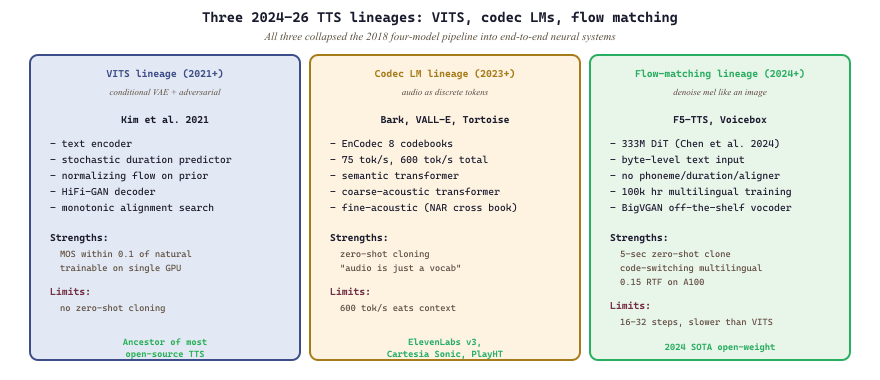
Text-to-speech (TTS) has crossed the uncanny valley. The pipeline of 2018 (text -> phonemes -> spectrogram -> vocoder, four separate models) has collapsed into single end-to-end systems that map characters or tokens directly to waveform-quality audio. Three lineages dominate: VITS-style conditional VAEs with adversarial training, codec language models (Bark, VALL-E, Tortoise) that treat audio as a sequence of discrete tokens, and flow-matching models (F5-TTS, Voicebox) that denoise mel-spectrograms in the same way image diffusion models denoise pixels. All three families share one architectural lesson from the rest of this book: stack transformer blocks on top of a learned audio representation, and the same recipe that produces ChatGPT produces Cartesia Sonic. This section is the foundation for everything that follows in Chapter 20: cloning (Section 20.2), music (Section 20.3), editing (Section 20.4), and ASR (Section 20.5).
Prerequisites
This section assumes the transformer mechanics from Section 3.1, the tokenization and vocabulary discussion from Section 1.6, and the autoregressive next-token loss from Section 6.2. A brief detour through diffusion-model basics (the image variant covered in Section 19.7) helps with the flow-matching half of the section.
20.1.1 From Tacotron to End-to-End Neural TTS
Modern TTS has three jobs: convert text into a phonetic plan, predict an acoustic feature sequence (typically a mel-spectrogram or a stream of audio codec tokens), and turn that feature sequence into a waveform. Before 2021, each job was a separate neural network. Tacotron 2 (Shen et al., 2018) handled text-to-spectrogram with an attention-based seq2seq, and a WaveNet or HiFi-GAN vocoder turned the spectrogram into 16-bit PCM samples at 22 or 24 kHz. The cracks in this pipeline showed at the seams: training data mismatch between modules, exposure bias when the spectrogram predictor saw its own outputs at inference, and a long tail of failure modes where the attention would skip or repeat words.
The end-to-end shift fused these stages. VITS (Kim et al., 2021) trained the text encoder, the duration predictor, the latent z-sequence, and a HiFi-GAN-style decoder jointly using a variational lower bound plus an adversarial loss. The model never explicitly emits a spectrogram at inference; the latent z passes straight into the GAN-trained decoder, and you read waveform out the other end. This eliminated the mismatch problem and pushed the mean opinion score (MOS) within 0.1 of natural recordings on LJSpeech.
In Section 22.1 a tokenizer maps text into discrete IDs that a transformer can consume. The 2023-2024 generation of TTS uses the same idea for audio: a neural codec (EnCodec, SoundStream, Mimi, DAC) compresses 24 kHz audio into 50 to 75 discrete tokens per second across 4 to 32 residual codebooks, and a transformer language model is trained to predict the next codec token given text. Bark, VALL-E, and Tortoise are all instances of this recipe; their differences are which codec, how many codebooks they autoregress, and how much data they trained on. Once you internalize that audio is just another vocabulary, every trick you know about LLM training (KV caching, FlashAttention, RoPE) transfers wholesale.
20.1.2 VITS: The Flow-Based End-to-End Baseline
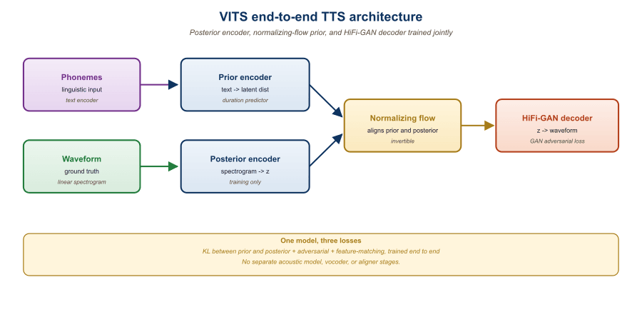
VITS (Variational Inference with adversarial learning for end-to-end Text-to-Speech) is the architectural ancestor of most open-source neural TTS in 2026. It treats speech generation as a conditional VAE problem with four core modules: a text encoder that produces a sequence of phoneme-level latents, a stochastic duration predictor that decides how long each phoneme should last, a normalizing flow that transforms the text-conditioned prior into a more expressive distribution over the latent z (so that the prior can match the richer posterior), and a HiFi-GAN decoder that maps z directly to waveform. The clever piece is the monotonic alignment search (MAS): a non-differentiable dynamic-programming routine inside the training loop that finds the best phoneme-to-frame alignment, eliminating the need for an external aligner like Montreal Forced Aligner.
The training objective combines a reconstruction loss on the waveform (mel-spectrogram L1 plus multi-period and multi-scale discriminators), a KL divergence between the prior and the posterior over z, and a duration loss over the phoneme-level durations. The result is a single network that takes characters or phonemes in and produces 24 kHz audio out, trainable on a single GPU in a few days on a dataset like LJSpeech.
The VITS training objective is a conditional variational lower bound augmented with HiFi-GAN adversarial and feature-matching losses. Writing $x$ for the waveform, $c$ for the phoneme sequence, $z$ for the latent acoustic representation, $q(z \mid x)$ for the posterior encoder, and $p(z \mid c)$ for the text-conditional prior (text encoder followed by a normalizing flow), the loss is
where the first term is the HiFi-GAN reconstruction term, the KL pulls the text-conditional prior toward the posterior given the speech, $\mathcal{L}_\mathrm{dur}$ trains the stochastic duration predictor (a normalizing flow on phoneme durations), and the last two are the adversarial and feature-matching losses on the synthesized waveform $\hat{x}$. The KL is computed with respect to the monotonic alignment search (MAS) result, which finds the discrete alignment between phonemes and latent frames that maximizes the prior likelihood given the posterior sample. Because MAS is non-differentiable, the discrete alignment is treated as a stop-gradient hard target and gradients flow only through $q$ and the flow.
from TTS.api import TTS
import torch

# Pretrained VITS on LJSpeech (single English speaker, 22 kHz).
device = "cuda" if torch.cuda.is_available() else "cpu"
tts = TTS(model_name="tts_models/en/ljspeech/vits", progress_bar=False).to(device)

# Direct waveform synthesis: text in, 22 kHz float waveform out.
wav = tts.tts(text="The quick brown fox jumps over the lazy dog.")
print(len(wav), "samples", f"({len(wav) / 22_050:.2f} s at 22 kHz)")
# 71680 samples (3.25 s at 22 kHz)

tts.tts_to_file(text="VITS skips spectrograms entirely.", file_path="out.wav")

# Multi-speaker variant: pick speaker by name from the speaker list.
vctk = TTS("tts_models/en/vctk/vits", progress_bar=False)
vctk.tts_to_file(text="Hello world.", speaker="p225", file_path="p225.wav")Compare VITS to the Tacotron 2 + HiFi-GAN baseline on the LJSpeech benchmark. For a 5-second target utterance (about 25 phonemes, 215 mel frames at 22 kHz), Tacotron 2's autoregressive decoder emits one mel frame per step at roughly 700 frames/second on an RTX 4090, taking about 0.31 s, plus HiFi-GAN's roughly 0.05 s vocoder pass, for a total of about 0.36 s (real-time factor 0.072). VITS runs the entire stack in a single feed-forward pass (text encoder about 5 ms, flow about 8 ms, duration predictor about 2 ms, decoder about 35 ms) for roughly 50 ms total, a real-time factor of 0.010, around 7x faster than the Tacotron 2 pipeline. On naturalness, the published LJSpeech MOS is 4.43 for VITS versus 4.43 for ground-truth recordings (statistically indistinguishable within a 0.05 confidence interval), 4.07 for Tacotron 2 + HiFi-GAN, and 4.05 for FastSpeech 2 + MelGAN. An end-to-end model matching natural recordings on a controlled single-speaker corpus is what put VITS in the architectural foundation of XTTS, YourTTS, VITS-2, and most open-source TTS systems shipped between 2021 and 2026.
20.1.3 Bark and Codec Language Models
Suno AI's Bark (released April 2023) sits in a different lineage. Instead of a VAE plus flow, it is a stack of transformer decoders that autoregress over audio codec tokens. Bark uses EnCodec at 24 kHz with 8 residual codebooks, producing 75 tokens per second per book, or 600 tokens per second of audio total. The model decomposes this into three stages: a semantic transformer that predicts a coarse stream of semantic tokens (derived from a quantized HuBERT-like model), a coarse-acoustic transformer that predicts the first two EnCodec codebooks conditioned on the semantic stream, and a fine-acoustic transformer that fills in codebooks 3 through 8 conditioned on the first two. The fine model is non-autoregressive across codebooks but autoregressive across time.
This staged decomposition matters because audio is exquisitely high-dimensional. A naive flat autoregression over 600 tokens per second of 24 kHz speech would consume the entire context window of GPT-4 in 13 seconds of audio. Splitting semantics from acoustics, and coarse from fine, lets each stage operate at a manageable rate.
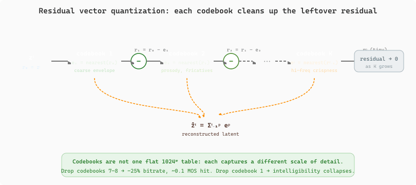
The "8 codebooks at 75 Hz" recipe that powers Bark, VALL-E, and Moshi is a Residual Vector Quantizer (RVQ) bolted onto a convolutional encoder-decoder. The encoder is a stack of strided 1D convolutions: input 24 kHz waveform $\mathbf{w} \in \mathbb{R}^{T}$, output latent $\mathbf{z} \in \mathbb{R}^{T/320 \times d}$ at $d = 128$ channels. The 320x downsampling lands the frame rate at exactly 75 Hz for 24 kHz audio. The RVQ then quantizes each latent vector $\mathbf{z}_t$ with a chain of $K$ codebooks $\{\mathcal{C}_1, \ldots, \mathcal{C}_K\}$, each containing 1024 entries of dimension $d$. The chain quantizes the running residual:
The key property is that $K$ residual codebooks of size 1024 do not behave like a single flat codebook of size $1024^K$: each codebook captures a different scale of detail. Codebook 1 typically encodes the coarse spectral envelope (vowel quality, pitch register), codebook 2 captures finer prosodic and fricative detail, and later codebooks fill in the high-frequency noise components that affect perceived crispness. This is why low-bandwidth applications often drop the last few codebooks: dropping codebooks 7 and 8 cuts bitrate by 25% with a 0.1 MOS hit, while dropping codebook 1 destroys intelligibility.
Training combines a perceptual reconstruction loss (multi-scale STFT plus L1 on time-domain samples), an adversarial loss from multi-period and multi-scale discriminators (Defossez et al. use HiFi-GAN-style discriminators), and a commitment loss $\sum_k \lVert \mathrm{sg}(e_k) - r_{k-1} \rVert_2^2$ that pulls each residual toward its assigned codebook entry (the $\mathrm{sg}$ is the stop-gradient operator that prevents the codebook itself from chasing the encoder). To avoid dead codebook entries, EnCodec uses exponential-moving-average updates (each entry tracks the mean of its assigned latents with EMA decay 0.99) and a "random restart" for any entry that goes unused for too long. Mimi (Defossez et al., 2024) adds a critical twist: it freezes the first codebook of its RVQ and trains it with a distillation loss against a frozen WavLM/HuBERT encoder, so codebook 1 carries explicit semantic content. This is what makes Moshi a true speech-to-speech model: the first codebook stream is a clean semantic representation that the language model can reason over, and codebooks 2 through 8 carry the prosody and timbre needed for naturalistic synthesis. References: Defossez et al., "High Fidelity Neural Audio Compression" (EnCodec), arXiv:2210.13438 (2022); Zeghidour et al., "SoundStream," arXiv:2107.03312 (2021); Defossez et al., "Moshi," arXiv:2410.00037 (2024).
Figure 20.1.3 unrolls the residual chain: each codebook quantizes what the previous codebooks could not capture, so the running residual $r_k = r_{k-1} - e_k$ shrinks from coarse spectral envelope down to fine high-frequency detail across the $K$ stages.
The Bark recipe (or a close cousin) ships behind several popular voice products. ElevenLabs v3 (2024) is a closed-weights codec LM with proprietary improvements in expressivity and pacing. Cartesia Sonic (2024-2025) replaces the transformer backbone with a state-space model (Mamba-2 derivative) to achieve sub-100 ms time-to-first-byte on streaming TTS. PlayHT 2.0 ships a multilingual codec LM with voice cloning. Open-source Bark itself remains the cheapest way to prototype any codec-LM-based product without negotiating API keys.
20.1.4 F5-TTS: Flow Matching Meets TTS
F5-TTS (Chen et al., 2024, arXiv:2410.06885) is the 2024 state of the art in zero-shot open-weight TTS. It abandons both VAE and codec-LM lineages in favor of a flow-matching transformer that denoises mel-spectrograms conditioned on text. The "F5" in the title stands for "A Fairytaler that Fakes Fluent and Faithful Speech with Flow Matching" (five F-words; the authors lean into the pun). It is a 336M-parameter DiT (Diffusion Transformer; see Section 33.1 for the video DiT variant) trained on the Emilia multilingual dataset (~95k hours).
The architectural simplification is striking. F5-TTS has no phoneme tokenizer, no duration predictor, no alignment search, and no vocoder beyond an off-the-shelf BigVGAN. Text is byte-level. Audio conditioning at inference (the reference voice clip) is concatenated with masked target frames, and the DiT learns to fill in the missing mel frames given the text. Inference is 16 to 32 flow-matching steps, similar in cost to Stable Diffusion 3 at the same parameter count. The model handles zero-shot voice cloning from a 5-second prompt out of the box, code-switches between languages, and runs at roughly 0.15 real-time factor on a single A100.
# Synthesizing speech with Bark (Suno-AI's open-source codec LM)
# pip install bark
from bark import SAMPLE_RATE, generate_audio, preload_models
from scipy.io.wavfile import write as write_wav

# Download and cache the three transformer stages (semantic, coarse, fine).
# First call pulls ~5 GB; subsequent calls are local.
preload_models()

# Bark supports inline tags: [laughs], [sighs], [music], (whispering),
# as well as multilingual text and a small set of curated "history prompts".
prompt = (
    "Hello, my name is Suno. And, uh, I like pizza. [laughs] "
    "But I also like other things, like reading books and watching films."
)

audio_array = generate_audio(prompt, history_prompt="v2/en_speaker_6")
write_wav("bark_output.wav", SAMPLE_RATE, audio_array)
print(f"Generated {len(audio_array) / SAMPLE_RATE:.1f} seconds at {SAMPLE_RATE} Hz")bark library. The history_prompt selects from Suno's curated voice library; pass None to sample a random voice instead. Bark is unique among open TTS in supporting nonverbal sounds ([laughs], [sighs]) directly in the prompt because its semantic transformer was trained on transcripts that include them.20.1.5 Prosody, Multi-Speaker, and Emotion Control
Naturalness is no longer the bottleneck; expressivity is. The 2024-2026 generation of TTS competes on prosody (pitch contour, stress, pacing), emotion (calm, angry, sad, excited), and speaker fidelity in multi-speaker contexts. There are four main control mechanisms in production.
The first is speaker embeddings, where a separate speaker-verification network (a wav2vec-XLSR or a similar self-supervised model) produces a 256-to-512-dimensional vector that conditions the TTS decoder. This is how VITS-2 and YourTTS extend single-speaker models to multi-speaker zero-shot synthesis. The second is reference-prompt conditioning, where a clip of target audio is concatenated with the input mel and the model learns to copy the style; F5-TTS, VALL-E, and NaturalSpeech 3 all use this trick. The third is natural-language style prompts: PromptTTS and Audiobox accept text like "an angry old man speaking quickly with a slight British accent" alongside the content text. The fourth is fine-grained controls exposed at inference: ElevenLabs v3 ships an "emotion" slider and a "stability" slider that act as classifier-free guidance weights on internal style channels.
The most common TTS production bug is treating the emotion slider as if it composes with itself. Setting "stability=0.1, similarity=0.9" gives a different output distribution than "stability=0.9, similarity=0.1", but neither is necessarily what a director means by "more angry, less crisp." Always A/B at least three random seeds per slider configuration when shipping a new voice; the variance across seeds at fixed sliders is often larger than the effect of moving a slider by a quarter.
20.1.6 The 2026 TTS Landscape: Open vs. Commercial
The commercial-open gap on raw audio quality is narrower than on most other modalities, but production reliability still favors the API vendors. Figure 20.1.4 summarizes the field as of late 2025.
| Model | Year | License | Zero-Shot Clone | Languages | Streaming Latency |
|---|---|---|---|---|---|
| F5-TTS | 2024 | CC-BY-NC 4.0 (weights) | 5 s reference | Multilingual (Emilia) | Batch only |
| Bark | 2023 | MIT | Limited (preset voices) | 13 languages | ~3 s (offline) |
| VITS-2 / XTTS-v2 | 2023 | CPML (XTTS) | 6 s reference | 16 languages | ~500 ms |
| ElevenLabs v3 | 2024 | Closed API | 30 s pro clone | 32 languages | ~250 ms first byte |
| Cartesia Sonic | 2024 | Closed API | 3 s reference | 15 languages | ~75 ms first byte |
| PlayHT 3.0 | 2025 | Closed API | 10 s reference | 40 languages | ~200 ms first byte |
| OpenAI tts-1-hd | 2024 | Closed API | No (6 preset voices) | Multilingual | ~400 ms first byte |
# Comparison: F5-TTS zero-shot synthesis (open weights, mel + flow matching)
# pip install f5-tts
from f5_tts.api import F5TTS

f5 = F5TTS(
    model_type="F5-TTS",            # or "E2-TTS" for the smaller variant
    vocoder_name="vocos",           # 24 kHz, BigVGAN also supported
)

# Reference clip + its transcript anchor the voice and prosody.
# Five seconds of clean speech is enough; longer hurts more than it helps.
ref_audio = "alice_5sec.wav"
ref_text = "Hello, this is Alice and I am testing the synthesis system."

target_text = (
    "The flow matching denoiser inside F5-TTS predicts the velocity "
    "of the mel-spectrogram, not the spectrogram directly."
)

wav, sr, _ = f5.infer(
    ref_audio=ref_audio,
    ref_text=ref_text,
    gen_text=target_text,
    nfe_step=32,                     # number of flow-matching steps
    cfg_strength=2.0,                # classifier-free guidance scale
    speed=1.0,
)
import soundfile as sf
sf.write("f5_output.wav", wav, sr)
print(f"Generated {len(wav) / sr:.1f}s at sr={sr}")nfe_step trades quality for latency in the same way num_inference_steps does in Stable Diffusion. The model handles cross-lingual transfer if gen_text is in a different language than ref_text.20.1.7 Prosody from an LLM: The Emerging Pattern
A 2025 architectural trend that will dominate 2026 is using an LLM to generate the prosody plan and only delegating the acoustics to the TTS model. The pipeline looks like: (1) GPT-4o or Claude takes the text and an instruction ("read this as if you are calming a child after a nightmare"), and emits the same text annotated with SSML-like tags for pacing, emphasis, and emotion shifts; (2) a smaller TTS model (Cartesia or F5-TTS) executes that prosody plan. The factorization is appealing because the LLM already knows narrative pacing, sarcasm, and dialogue structure from its pretraining corpus, while the acoustic model has a much narrower job. Audiobox (Meta, 2023) and Voicebox (Meta, 2023) prototyped this with end-to-end joint training, but the production pattern of the API era is to keep the LLM and the TTS as separate services and rely on a structured intermediate representation between them.
F5-TTS at int8 quantization fits in 333 MB of weights and runs on a M2 MacBook. The same architecture that requires a data center to serve at ElevenLabs scale (50k concurrent streams, sub-100 ms TTFB) is, at the model-weights level, smaller than a single Premiere Pro render. The constraint is throughput, not capability.
Three TTS lineages cover the field: VITS-style VAE-flow for tight end-to-end training on bounded data, codec language models like Bark for prompt-driven expressivity at the cost of latency, and flow-matching DiTs like F5-TTS for zero-shot cloning with simple architectures. Commercial APIs (ElevenLabs, Cartesia, PlayHT) wrap one of these recipes behind sub-second TTFB streaming, multilingual coverage, and SLAs that open weights cannot match. The acoustic gap is small; the production gap is real.
Show Answer
Show Answer
Show Answer
In the next section, Section 20.2: Voice Cloning, Zero-Shot TTS, and Voice Conversion, we continue.
What Comes Next
Section 20.2 takes the zero-shot cloning capability of F5-TTS and asks the harder question: when is cloning a person's voice a consent violation, and how do we build pipelines that respect that boundary while still letting users dub their own audiobooks? After that, Section 20.3 pivots from speech to music: the same codec-LM and flow-matching ideas that produce ElevenLabs and F5-TTS also produce Suno and Udio.
Further Reading
- Kim, J., Kong, J., & Son, J. (2021). Conditional Variational Autoencoder with Adversarial Learning for End-to-End Text-to-Speech. ICML 2021. arXiv:2106.06103. The VITS paper that established end-to-end neural TTS.
- Chen, Y. et al. (2024). F5-TTS: A Fairytaler that Fakes Fluent and Faithful Speech with Flow Matching. arXiv:2410.06885. The state-of-the-art open-weight zero-shot TTS system at the time of writing.
- Suno AI (2023). Bark. github.com/suno-ai/bark. The reference codec-LM TTS implementation; MIT-licensed weights and inference code.
- Wang, C. et al. (2023). Neural Codec Language Models are Zero-Shot Text-to-Speech Synthesizers (VALL-E). arXiv:2301.02111. Microsoft's three-second prompt cloning system; the first prominent codec-LM TTS.
- Le, M. et al. (2023). Voicebox: Text-Guided Multilingual Universal Speech Generation at Scale. NeurIPS 2023. arXiv:2306.15687. Meta's flow-matching TTS that pioneered the F5 lineage.
- Cartesia AI (2024). Sonic: Mamba-Based State-Space TTS for Real-Time Conversational AI. cartesia.ai/blog/sonic. The first production codec-LM-style TTS built on state-space models instead of transformers.
- ElevenLabs (2024). v3 Technical Notes and Voice Library. elevenlabs.io/docs. The commercial reference for expressive multilingual TTS in 2024-2025.
- OpenAI (2024). Audio API: tts-1 and tts-1-hd. platform.openai.com/docs/guides/text-to-speech. The simplest production TTS endpoint, useful as a low-friction baseline.