"I learned to read a wrist camera in three weeks. Learning what to do with a wrist camera took the other 47."
A Vision-Language-Action (VLA) model is, in one sentence, a multimodal LLM whose vocabulary has been extended with motor tokens so the same softmax that picks "Paris" given "The capital of France is" picks a robot joint angle given a wrist-camera image and the instruction "place the red block on the plate". This section nails down the single equation that defines VLAs, walks through action tokenization as the engineering trick that makes it work, and explains why every architectural primitive you absorbed from the text-only transformer transfers without modification to the embodied setting.
Prerequisites
This section assumes the next-token factorization from Section 6.2, the multimodal token-fusion patterns from Section 22.7, and a working intuition for KV cache mechanics from Section 9.4.
24.1.1 The VLA Equation
OpenVLA's reference implementation by Stanford and Toyota Research (Kim et al., 2024) is exactly 1,792 motor-bin tokens added to a standard Llama-2-7B vocabulary, chosen because 1,792 is divisible by 256 (8 dimensions x 256 bins for the WidowX arm). The choice of 256 bins per dimension was reportedly because "that's how many colors fit in a byte", a digital-graphics joke that escaped into a robotics paper.
A VLA models a single conditional distribution. Let I denote the multi-view image stack the robot's cameras produce at a timestep (typically a wrist-mounted view plus a third-person view), let \ell denote the natural-language instruction, and let a_{1:H} denote the action chunk the policy must emit over a horizon of H control steps. The VLA factorizes the action distribution autoregressively:
p_theta(a_{1:H} | I, l) = prod_{t=1..H} p_theta(a_t | I, l, a_{1:t-1})Read that equation carefully. The right-hand side is exactly the next-token factorization from Section 6.2, with two differences that are not changes to the math: (a) the conditioning context contains image tokens in addition to text tokens, and (b) the symbols being predicted are drawn from a vocabulary slice reserved for motor commands. Everything that follows in this chapter is engineering glue around that single factorization.
Replace "vocabulary of 50k BPE pieces" with "vocabulary of 50k BPE pieces plus 1,792 motor bins". Replace "user message" with "front-camera image, wrist-camera image, instruction string". Replace "assistant message" with "an action chunk that decodes into joint deltas". The transformer trunk, the KV cache, the cross-entropy loss, FlashAttention, RoPE, and speculative decoding all transfer with zero source changes. If you can read the GPT-2 reference implementation, you can read the OpenVLA reference implementation.
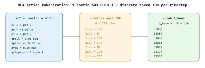
24.1.2 Action Tokenization: BPE for the Body
The crux of "extend the vocabulary with motor tokens" is making a discrete vocabulary out of a continuous motor signal. Robots in the manipulation regime have somewhere between 6 and 14 controllable degrees of freedom (DOF). For a single-arm manipulator with a gripper, the action vector is 7-dimensional: three Cartesian deltas (dx, dy, dz), three rotation deltas (droll, dpitch, dyaw), and one gripper signal (open or close). The action tokenizer quantizes each dimension into K bins (RT-2 and OpenVLA both use K=256) and assigns a unique vocabulary index to each bin of each dimension. Seven DOF times 256 bins gives 1,792 reserved indices, a rounding error against a 32k or 128k text vocabulary.
Formally, the per-dimension quantization is uniform over the action range observed in training data:
where $\mathrm{lo}_d, \mathrm{hi}_d$ are the 1st and 99th percentiles of action dimension $d$ in the training set, $V_{\text{base}}$ is the first reserved vocabulary index (often the start of a "least-used" range of an existing BPE vocabulary), and $K = 256$. Decoding inverts the bin and indexes back into the dimension via $d = \lfloor (\text{token} - V_{\text{base}}) / K \rfloor$ and $b = (\text{token} - V_{\text{base}}) \bmod K$.
The forward pass produces seven action tokens per timestep, decoded by inverting the quantization:
import numpy as np

class ActionTokenizer:
    """7-DOF end-effector tokenizer (OpenVLA / RT-2 convention).

    Each dimension is quantized into K bins. Bin index b for dimension d
    maps to vocabulary index   vocab_base + d * K + b.
    """

    def __init__(self, vocab_base: int = 31744, n_bins: int = 256, n_dof: int = 7):
        self.vocab_base = vocab_base
        self.n_bins = n_bins
        self.n_dof = n_dof
        # Per-dimension normalization derived from training-data quantiles.
        self.lo = np.array([-0.05, -0.05, -0.05, -0.4, -0.4, -0.4, 0.0])
        self.hi = np.array([ 0.05,  0.05,  0.05,  0.4,  0.4,  0.4, 1.0])

    def encode(self, action: np.ndarray) -> np.ndarray:
        x = np.clip((action - self.lo) / (self.hi - self.lo), 0.0, 1.0)
        bins = np.floor(x * (self.n_bins - 1)).astype(np.int32)
        return self.vocab_base + np.arange(self.n_dof) * self.n_bins + bins

    def decode(self, tokens: np.ndarray) -> np.ndarray:
        offset = tokens - self.vocab_base
        bins = offset % self.n_bins
        x = bins.astype(np.float32) / (self.n_bins - 1)
        return self.lo + x * (self.hi - self.lo)

tok = ActionTokenizer()
a = np.array([0.02, -0.01, 0.03, 0.0, 0.1, -0.2, 1.0])
ids = tok.encode(a)
print(ids)          # 7 vocabulary indices, all in [31744, 33535]
print(tok.decode(ids)) # roughly equal to a, modulo 1/256 quantizationTreating actions as discrete tokens, rather than regressing continuous values, lets the policy emit multimodal distributions. If two valid grasps lie 10 cm apart, a Gaussian regression head averages them and the gripper crashes between objects. A categorical softmax happily puts mass on both bins, and sampling picks one. This is why nucleus sampling and beam search from Chapter 4 transfer to robotics: choosing among multimodal trajectories is the same problem as choosing among multimodal sentence continuations.
24.1.3 The End-to-End Policy
The full forward pass strings four off-the-shelf components together. A vision encoder (SigLIP, DINOv2, or a fused pair) consumes each camera view and emits a sequence of image-patch tokens. The instruction string is tokenized by the LLM's existing BPE tokenizer. The two streams are interleaved with a small set of separator tokens and fed into a decoder-only transformer. The LM head produces logits over the unified text-plus-action vocabulary. At inference time you greedy-decode (or low-temperature sample) seven tokens, run them through the inverse action tokenizer, and ship the resulting 7-D vector to the robot's low-level controller.
| Stage | Input | Output | Reused from text LLM? |
|---|---|---|---|
| Vision encoder | Multi-view images | ~256 patch tokens | Yes (ViT / SigLIP) |
| Text tokenizer | Instruction string | ~32 BPE tokens | Yes (LLaMA BPE) |
| Transformer trunk | Interleaved token sequence | Hidden states | Yes (LLaMA 7B/13B) |
| LM head | Last hidden states | Vocab logits (text + action) | Yes (Linear + softmax) |
| Action detokenizer | 7 sampled token IDs | 7-D end-effector delta | No (the only new piece) |
The reference pseudocode for a single control step is short enough to fit on one screen:
def vla_step(model, tokenizer, action_tokenizer,
             wrist_img, third_img, instruction):
    # 1. Encode vision and text into a unified token sequence.
    v_tokens = model.vision_encoder([wrist_img, third_img])
    t_tokens = tokenizer.encode(f"In: {instruction}\nOut:")
    prefix = torch.cat([v_tokens, t_tokens], dim=1)

    # 2. Greedy-decode exactly n_dof tokens from the action slice.
    action_ids = []
    past = None
    inputs = prefix
    for d in range(action_tokenizer.n_dof):
        out = model(inputs, past_key_values=past)
        past = out.past_key_values
        logits = out.logits[:, -1]
        # Mask the logits to the slice for dimension d (forces a valid action token).
        lo = action_tokenizer.vocab_base + d * action_tokenizer.n_bins
        hi = lo + action_tokenizer.n_bins
        tok_id = lo + logits[:, lo:hi].argmax(dim=-1)
        action_ids.append(tok_id)
        inputs = tok_id.unsqueeze(-1)

    # 3. Detokenize seven IDs into a 7-D end-effector delta.
return action_tokenizer.decode(torch.stack(action_ids).cpu().numpy())24.1.4 Action Chunking and Receding-Horizon Control
Predicting one action and immediately running it round-trips through the network at every control step, which the bottleneck is the transformer forward pass. The fix is action chunking: predict an entire horizon a_{1:H} at once, execute the first few, and re-plan. This is the receding-horizon pattern from classical model-predictive control, except the model is a 7B-parameter transformer instead of a 50-line MPC solver. Chunking lets a policy that forward-passes at 5-10 Hz nevertheless emit smooth 30 Hz control by interpolating between the predicted waypoints.
If H=8 and you forward-pass at 5 Hz, the robot follows an open-loop trajectory for 1.6 seconds before the next replan. A human walking into the workspace during that window will be hit by an obstacle-blind robot. Production VLAs at 2026 robotics startups (Physical Intelligence, Skild, Figure) typically set H so the replan period is at most 200 ms and pair the policy with a separate reactive safety layer that can halt execution mid-chunk. The chunking knob trades smoothness against reactivity.
24.1.5 Where the Equation Lives in the Broader Stack
The factorization p_theta(a_{1:H} | I, l) sits at the lowest layer of a three-tier robotics stack that you will see repeatedly through Chapters 39 and 40. At the top is a planning LLM (covered in Section 24.7 on SayCan and Section 24.8 on Code-as-Policies) that decomposes a high-level instruction like "tidy the kitchen" into subgoals. In the middle is the VLA policy that turns each subgoal plus current pixels into actions. At the bottom is a 1 kHz low-level controller (PID, impedance, or operational-space) that turns the VLA's coarse 7-D commands into 1 kHz joint torques. Most of this chapter focuses on the middle layer; the top layer is Chapter 39's job; the bottom layer lives in textbooks on classical control and is, refreshingly, mostly unchanged by the LLM revolution.
| Layer | Rate | Input | Output | Implementation |
|---|---|---|---|---|
| Planner LLM | 0.1-1 Hz | Goal + context | Subgoal sequence | GPT-4o, Claude, Gemini via API |
| VLA policy | 5-20 Hz | Subgoal + pixels | End-effector deltas | OpenVLA, pi-0, RT-2-X |
| Low-level controller | 500-1000 Hz | Deltas + state | Joint torques | Operational-space PID |
The discrete-token formulation in Section 1 is one of two dominant approaches in 2026 VLAs. The other is the diffusion policy, where p_theta(a_{1:H} | I, l) is parameterized by a denoising network and sampled by iterative refinement instead of autoregressive decoding. Physical Intelligence pi-0 (covered in Section 24.3) uses flow matching, a close cousin of diffusion that produces continuous-valued actions directly without binning. The two formulations are equivalent in expressive power but make different trade-offs on inference latency, training stability, and the smoothness of emitted trajectories. The empirical picture in 2026 is that both work; the choice is driven by team familiarity and inference-stack preferences more than by hard performance gaps.
24.1.6 Why the Text Vocabulary Survives Action Finetuning
A reasonable worry: extending the vocabulary with motor bins and finetuning on robot data should catastrophically forget the text capabilities of the base LLM. Empirically, this does not happen, for two reasons. First, the text vocabulary is orders of magnitude larger than the action vocabulary, so the gradient pressure on text tokens from action-data batches is small. Second, the standard recipe (RT-2, OpenVLA, pi-0) is to co-train on a mix of robot demonstrations and a small fraction of text-only and vision-language data; this regularizes the trunk. The practical consequence is that a VLA can still hold a conversation about the scene it sees, which is the substrate that makes "explainable robot actions" a feature rather than a research aspiration. You can ask the policy "why did you grasp the cup that way?" mid-trajectory and get a coherent answer from the same model that is also emitting motor tokens.
A VLA trained on one robot's action space (say, the WidowX 7-DOF end-effector) does not transfer to another robot's action space (say, a 6-DOF arm with a different gripper convention) without retokenization and at least light finetuning. The action vocabulary is robot-specific. The cross-embodiment generalization that RT-2-X and pi-0.5 promise (Section 24.3, Section 24.4) is delivered by training on data from many robots with a unified action space, not by zero-shot vocabulary reuse. Mixing this up costs robotics startups months of debugging time when they expand from one hardware platform to a second.
Key Takeaway
A VLA is fully specified by one equation, p_theta(a_{1:H} | I, l) = prod_t p_theta(a_t | I, l, a_{1:t-1}), which is the same next-token factorization that defines text LLMs. The only new engineering piece is action tokenization, a 30-line module that quantizes continuous motor commands into a vocabulary slice. Everything else, vision encoders, transformers, sampling, KV caches, transfers unchanged from the text-only stack. This is why robotics in 2026 hires LLM engineers rather than reinventing them.
Show Answer
Show Answer
Show Answer
logits = logits.masked_fill(~slice_mask, float('-inf')) where slice_mask marks only indices in [vocab_base + d * n_bins, vocab_base + (d+1) * n_bins). With that mask the argmax can never escape to a text token, even if the unconstrained probability for some BPE token is higher on a noisy input. This is the standard constrained-decoding pattern applied at the sampling step rather than at training time.Continue to Section 24.2: OpenVLA-7B Reference Implementation.
Section 24.1 gave you the equation; Section 24.2 opens the hood on OpenVLA-7B, the open-weights reference implementation that ships with PyTorch source you can run today. You will see the vision encoder choice (fused SigLIP+DINOv2), the training-data recipe (Open X-Embodiment), and the inference performance characteristics (about 6 Hz on an A100) in concrete code.