Pretraining Objectives & Paradigms

Tell a model to predict the next word and it learns grammar. Mask a word and it learns meaning. Corrupt a span and it learns to complain about the corruption, then fix it anyway.

Scale, Gleefully Predictive AI Agent

6.2.1 Causal Language Modeling (CLM)

Figure 6.2.1: Two pretraining objectives at the token level. Causal language modeling (left) predicts the next token from prior tokens only, the natural setup for autoregressive generation. Masked language modeling (right) hides random tokens and predicts them using bidirectional context, the natural setup for representation learning. Both objectives use the same Transformer backbone; only the attention mask and the loss differ.

Causal language modeling, also called autoregressive language modeling, trains a model to predict the next token given all previous tokens. Formally, given a sequence of tokens $x = (x_{1}, x_{2}, ..., x_{T})$, the model maximizes:

The model processes tokens left-to-right, with a causal attention mask that prevents each position from attending to future positions. This makes CLM naturally suited for text generation: at inference time, the model generates one token at a time, feeding each prediction back as input for the next step (see Section 4.1 for the mechanics of autoregressive decoding).

Why CLM Dominates Modern LLMs

Several properties make CLM the preferred objective for large-scale models:

• Every token is a training signal: Unlike MLM (which only learns from masked tokens), CLM provides a gradient signal at every position in the sequence, making training more sample-efficient.
• Natural generation: The training objective exactly matches the inference procedure, avoiding train-test mismatch.
• Scalability: The causal attention mask enables efficient KV caching during inference, where previously computed key-value pairs are reused (see Section 9.3 for KV cache optimization).
• Flexibility: The same model can be prompted for classification, generation, translation, and reasoning, all through the text completion interface. Chapter 12 covers the prompt engineering techniques that exploit this flexibility.

# Implementing causal language modeling loss from scratch
import torch
import torch.nn.functional as F
def causal_lm_loss(logits, labels):
    """
       logits: (batch, seq_len, vocab_size)
       labels: (batch, seq_len) - same as input tokens shifted by 1
       """
    # Shift: predict token t+1 from position t
    shift_logits = logits[:, :-1, :].contiguous()
    shift_labels = labels[:, 1:].contiguous()
    # Cross-entropy loss, ignoring padding tokens (label = -100)
    loss = F.cross_entropy(
        shift_logits.view(-1, shift_logits.size(-1)),
        shift_labels.view(-1),
        ignore_index=-100
    )
    return loss
# Example: batch of 2, sequence length 5, vocab size 100
logits = torch.randn(2, 5, 100)
labels = torch.randint(0, 100, (2, 5))
loss = causal_lm_loss(logits, labels)
print(f"CLM Loss: {loss.item():.4f}")
print(f"Perplexity: {torch.exp(loss).item():.2f}")

# Causal language modeling loss from scratch.
# Predict next token at each position; only the SHIFTED-LEFT targets contribute.
import torch
import torch.nn.functional as F

def causal_lm_loss(logits: torch.Tensor, input_ids: torch.Tensor) -> torch.Tensor:
    """logits: (batch, seq_len, vocab)
       input_ids: (batch, seq_len)
       Returns scalar cross-entropy averaged over all valid positions."""
    # Shift: predict input_ids[:, 1:] from logits[:, :-1, :]
    pred_logits = logits[:, :-1, :].contiguous()              # (B, T-1, V)
    targets     = input_ids[:, 1:].contiguous()               # (B, T-1)

    # Cross-entropy over flattened batch+positions
    loss = F.cross_entropy(
        pred_logits.view(-1, pred_logits.size(-1)),
        targets.view(-1),
    )
    return loss

# Quick sanity check
torch.manual_seed(0)
B, T, V = 2, 10, 50257
fake_logits = torch.randn(B, T, V)
fake_ids = torch.randint(0, V, (B, T))
print(f"Loss: {causal_lm_loss(fake_logits, fake_ids).item():.3f}")
# For an untrained random model on a 50K-token vocab, expect log(50257) ~= 10.8.

# Production equivalent: loss is computed internally
from transformers import AutoModelForCausalLM, AutoTokenizer
model = AutoModelForCausalLM.from_pretrained("gpt2")
tokenizer = AutoTokenizer.from_pretrained("gpt2")
inputs = tokenizer("The cat sat on the mat", return_tensors="pt")
outputs = model(**inputs, labels=inputs["input_ids"])
print(f"Loss: {outputs.loss.item():.4f}")

# Multi-token prediction: conceptual implementation
import torch
import torch.nn as nn
class MultiTokenPredictionHead(nn.Module):
    """N independent prediction heads sharing a transformer backbone."""
    def __init__(self, hidden_dim, vocab_size, n_heads=4):
        super().__init__()
        self.n_heads = n_heads
        # Each head: LayerNorm + Linear projection to vocab
        self.heads = nn.ModuleList([
            nn.Sequential(
            nn.LayerNorm(hidden_dim),
            nn.Linear(hidden_dim, vocab_size)
            )
            for _ in range(n_heads)
            ])
    def forward(self, hidden_states, labels):
        """
        hidden_states: (batch, seq_len, hidden_dim)
        labels: (batch, seq_len) - original token ids
        """
        total_loss = 0.0
        for k, head in enumerate(self.heads, start=1):
            logits = head(hidden_states) # (batch, seq_len, vocab)
            # Shift by k positions: predict token at t+k from position t
            shift_logits = logits[:, :-k, :].contiguous()
            shift_labels = labels[:, k:].contiguous()
            loss_k = nn.functional.cross_entropy(
                shift_logits.view(-1, shift_logits.size(-1)),
                shift_labels.view(-1),
                ignore_index=-100
                )
            total_loss += loss_k
            return total_loss / self.n_heads
            mtp = MultiTokenPredictionHead(hidden_dim=512, vocab_size=32000, n_heads=4)
            hidden = torch.randn(2, 128, 512)
            labels = torch.randint(0, 32000, (2, 128))
            loss = mtp(hidden, labels)
            print(f"MTP Loss (4 heads): {loss.item():.4f}")

6.2.2 Masked Language Modeling (MLM)

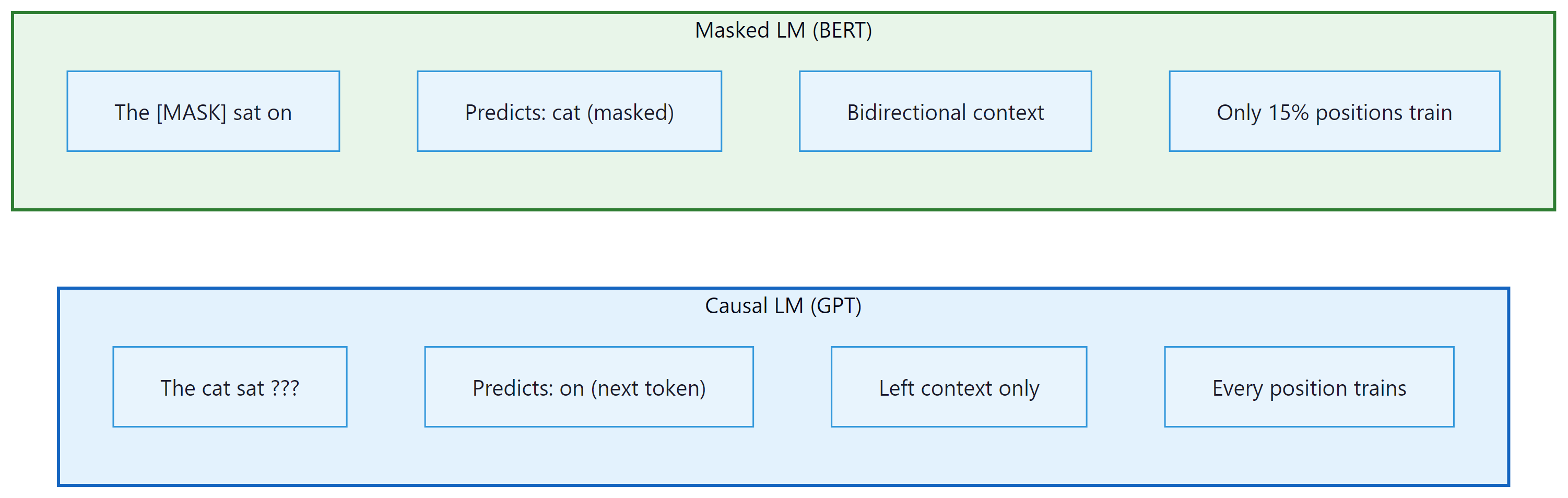
Masked language modeling, introduced by BERT, randomly masks a fraction of input tokens and trains the model to reconstruct them from the surrounding (bidirectional) context. The standard recipe masks 15% of tokens, with 80% replaced by [MASK], 10% replaced by a random token, and 10% kept unchanged.

where $M$ is the set of masked positions and $x_{\mathcal{M}}$ denotes the corrupted input (all tokens with masks applied).

Strengths and Limitations

MLM's bidirectionality is its greatest strength for understanding tasks. A model that sees both left and right context can build richer representations of each token. This is why BERT-style models dominate in classification, named entity recognition, and other tasks where the full context is available.

However, MLM has significant limitations. Only 15% of tokens provide training signal per forward pass, making it less sample-efficient than CLM. The [MASK] token never appears during inference, creating a train-test mismatch. And MLM models cannot naturally generate text because they assume access to future context during prediction.

Figure 6.2.2a: CLM sees only left context and trains on every token. MLM sees full context but trains only on masked positions.

CLM and MLM represent two ends of a spectrum: predict the next token versus predict masked tokens. But what if we masked entire spans of text rather than individual tokens? This hybrid idea led to a third family of pretraining objectives that combines the strengths of both approaches.

BERT's Joint Objective: MLM + Next Sentence Prediction

The original BERT was not trained on MLM alone. It optimized a joint loss combining masked language modeling with Next Sentence Prediction (NSP), a binary classification objective designed to teach the model relations between sentences. Each training example is a pair of segments $A$ and $B$ packed as [CLS] A [SEP] B [SEP], with the special [CLS] (classification) token prepended to the input and [SEP] separating the two segments. Half the time $B$ is the actual sentence that followed $A$ in the corpus, and half the time it is a random sentence drawn from elsewhere. A single binary classification head sitting on top of the context vector at the [CLS] position predicts whether $B$ is the true next sentence. The combined objective is:

The NSP loss is the standard binary cross-entropy on the [CLS] head, and the MLM loss is computed as before over the masked positions in the concatenated $A$ and $B$ sequence. The intent of NSP is to force the model to build a single context vector at the [CLS] position that summarizes the entire input, not just a single token's neighborhood. That summary is then directly usable as a sentence-pair (or single-sentence) representation for downstream tasks.

[CLS] as a Sentence Embedding (and Mean Pooling as an Alternative)

Because NSP trained the [CLS] context vector to encode the whole input, the natural recipe for using BERT as a sentence encoder is to take that single vector as the sentence embedding. Concretely, the post-training procedure for classification or retrieval is:

1. Tokenize the input as [CLS] tokens... [SEP].
2. Run a forward pass through BERT.
3. Read off the final-layer hidden state at position 0 (the [CLS] position). That vector is the sentence embedding.
4. Either feed it into a linear classifier head (fine-tuning), use it as a frozen feature, or compare two such vectors with cosine similarity for retrieval.

An equally common alternative is mean pooling: average the final-layer hidden states across all non-padding token positions to produce the sentence vector. Mean pooling often outperforms the raw [CLS] vector when the model was not specifically trained with NSP (for example, RoBERTa), and it is the default pooling strategy used in the Sentence-Transformers library (see Section 31.1 for sentence embeddings in retrieval, and Section 31.2 for the contrastive fine-tuning that turns raw [CLS] vectors into high-quality embeddings).

6.2.3 Span Corruption and Denoising Objectives

T5 introduced span corruption, a variant of MLM that masks contiguous spans of tokens rather than individual tokens. A random 15% of tokens are selected, grouped into contiguous spans, and each span is replaced with a single unique sentinel token (like <extra_id_0>). The model then generates the corrupted spans in order, separated by sentinel tokens.

Why Spans Are Better Than Single Tokens

Span corruption is more efficient than single-token masking for several reasons. First, the target sequence is shorter because multiple masked tokens are represented by a single sentinel, reducing the computational cost of the decoder. Second, the model must predict multiple consecutive tokens per span, encouraging it to learn phrase-level and sentence-level patterns rather than just word-level predictions.

# Simulating T5 span corruption
import random
def span_corruption(tokens, mask_ratio=0.15, mean_span_length=3):
    """Apply T5-style span corruption to a token list."""
    n = len(tokens)
    num_masked = int(n * mask_ratio)
    num_spans = max(1, num_masked // mean_span_length)
    # Generate random span starts and lengths
    mask = [False] * n
    masked_so_far = 0
    for _ in range(num_spans):
        if masked_so_far >= num_masked:
            break
            span_len = random.randint(1, mean_span_length * 2)
            start = random.randint(0, n - 1)
            for i in range(start, min(start + span_len, n)):
                mask[i] = True
                masked_so_far += 1
                # Build corrupted input and target
                corrupted, target = [], []
                sentinel_id = 0
                in_span = False
                for i, tok in enumerate(tokens):
                    if mask[i]:
                        if not in_span:
                            corrupted.append(f"<extra_id_{sentinel_id}>")
                            target.append(f"<extra_id_{sentinel_id}>")
                            sentinel_id += 1
                            in_span = True
                            target.append(tok)
                        else:
                            corrupted.append(tok)
                            in_span = False
                            return corrupted, target
                            tokens = "The quick brown fox jumps over the lazy dog".split()
                            random.seed(42)
                            corrupted, target = span_corruption(tokens)
                            print(f"Input:     {' '.join(corrupted)}")
                            print(f"Target:    {' '.join(target)}")

UL2: Mixture of Denoisers

UL2 (Unified Language Learning, 2022) took the denoising approach further by mixing multiple corruption strategies during pretraining. It combined three modes: (1) R-denoiser (regular denoising, like T5, with short spans), (2) S-denoiser (sequential denoising, similar to prefix LM, masking a suffix), and (3) X-denoiser (extreme denoising, with long spans and high mask ratios). A mode token prepended to each example tells the model which type of denoising to perform. This produced a single model that excelled at both understanding and generation tasks.

6.2.4 Prefix Language Modeling

Prefix LM is a hybrid approach used by models like PaLM and GLM. The input is divided into a prefix (which uses bidirectional attention) and a suffix (which uses causal attention). The prefix provides full context for encoding the input, while the suffix generates output autoregressively. This combines the encoding strength of MLM with the generation capability of CLM.

6.2.5 Fill-in-the-Middle (FIM)

Fill-in-the-middle is a training objective designed specifically for code models (like Codex, StarCoder, and CodeLlama, discussed further in Section 27.1). The key observation is that programmers frequently need to insert code at an arbitrary position within existing code, but standard CLM only supports appending tokens at the end.

FIM works by splitting a document into three parts: prefix, middle, and suffix. During training, these parts are rearranged so the model sees the prefix and suffix first, then generates the middle. The most common variant, called PSM (Prefix-Suffix-Middle), presents the input as:

An alternative variant, SPM (Suffix-Prefix-Middle), places the suffix before the prefix. The model learns to condition on both surrounding context to generate the infilling content.

# Fill-in-the-Middle (FIM) transformation
import random
def apply_fim(document, fim_rate=0.5, mode="PSM"):
    """Transform a document for FIM training."""
    if random.random() > fim_rate:
        return document # Keep as regular CLM with probability (1 - fim_rate)
    # Choose a random split point for the middle section
    chars = list(document)
    n = len(chars)
    split1 = random.randint(0, n)
    split2 = random.randint(split1, n)
    prefix = document[:split1]
    middle = document[split1:split2]
    suffix = document[split2:]
    if mode == "PSM":
        return f"<PRE>{prefix}<SUF>{suffix}<MID>{middle}"
    elif mode == "SPM":
        return f"<SUF>{suffix}<PRE>{prefix}<MID>{middle}"
    # Example with code
    code = """def fibonacci(n):
        if n <= 1:
            return n
        return fibonacci(n-1) + fibonacci(n-2)"""
    random.seed(0)
    fim_example = apply_fim(code, fim_rate=1.0)
    print(fim_example)

6.2.6 Multi-Token Prediction

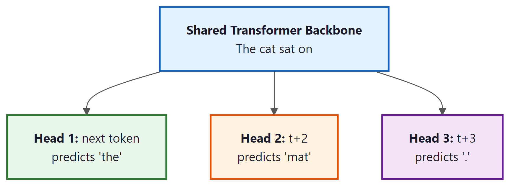
Standard CLM predicts only one token ahead. Multi-token prediction (MTP), introduced by Meta in 2024 and later adopted by DeepSeek V3, trains the model to predict several future tokens simultaneously. The architecture adds N independent prediction heads to a shared transformer backbone. Head k predicts token $x_{t+k}$ given tokens $x_{1}, ..., x_{t}$.

Why Predict Multiple Tokens?

The benefits of multi-token prediction are both theoretical and practical:

• Better representations: To predict multiple future tokens simultaneously, the model must encode richer information about the sequence at each position, including longer-range dependencies.
• Improved sample efficiency: Each training example provides N times more gradient signal per position.
• Speculative decoding compatibility: The additional prediction heads can be used as draft models for speculative decoding, accelerating inference by 2-3x without any additional model.
• Diminishing returns: Experiments show most of the benefit comes from N=4 heads. Adding more heads increases training memory without proportional gains.

Figure 6.2.4a: Multi-token prediction uses N independent heads on top of a shared backbone, each predicting a different future token.

# Multi-token prediction (Meta, "Better & Faster LLMs via Multi-Token Prediction" 2024).
# Train the model to predict the NEXT k tokens at every position, using k parallel heads.
# Improves sample efficiency and downstream code/math performance.
import torch
import torch.nn as nn
import torch.nn.functional as F

class MultiTokenPredictionHead(nn.Module):
    """k separate linear heads sharing the same trunk; head[i] predicts token (t+i+1)."""

    def __init__(self, d_model: int, vocab: int, n_future: int = 4):
        super().__init__()
        self.n_future = n_future
        self.heads = nn.ModuleList([nn.Linear(d_model, vocab) for _ in range(n_future)])

    def forward(self, hidden: torch.Tensor) -> list[torch.Tensor]:
        """hidden: (B, T, d_model) -> list of n_future tensors each (B, T, vocab)"""
        return [head(hidden) for head in self.heads]

    def loss(self, hidden: torch.Tensor, input_ids: torch.Tensor) -> torch.Tensor:
        """Sum cross-entropy across the k future positions, dropping the tail."""
        logits_list = self(hidden)
        B, T, _ = hidden.shape
        total = 0.0
        for i, logits in enumerate(logits_list, start=1):
            # head i predicts token at position (t+i); drop the last i positions
            valid_logits = logits[:, :T - i, :].contiguous().view(-1, logits.size(-1))
            targets      = input_ids[:, i:].contiguous().view(-1)
            total = total + F.cross_entropy(valid_logits, targets)
        return total / self.n_future

6.2.7 Continual Pretraining

All of the objectives described above focus on training a model from scratch. But a growing body of work demonstrates that continual pretraining (also called domain-adaptive pretraining or continued pretraining) is a powerful and cost-effective technique for adapting an existing foundation model to a new domain, language, or capability without the expense of a full training run.

The core idea is straightforward: take a pretrained model's checkpoint and resume CLM training on a new corpus that emphasizes the target domain. For example, a general-purpose model trained primarily on English web text can be continually pretrained on a large corpus of biomedical papers, legal documents, or code. The model retains its general capabilities while absorbing domain-specific knowledge, vocabulary patterns, and reasoning styles. This is far cheaper than pretraining from scratch because the model already has strong language understanding; the continual phase only needs to adjust the distribution, typically requiring 10 to 100 billion tokens rather than trillions.

Several practical considerations govern successful continual pretraining:

• Learning rate: The peak learning rate should be significantly lower than the original pretraining rate (typically 10 to 50% of the original). Starting with too high a rate causes catastrophic forgetting of the model's existing knowledge. Most practitioners use a WSD or cosine schedule with a short warmup phase.
• Data mixing: Mixing domain-specific data with a proportion of general data (often called "replay" data) helps prevent the model from losing its general capabilities. A common ratio is 70 to 90% domain data and 10 to 30% general replay data.
• Tokenizer adaptation: If the target domain uses specialized vocabulary (medical terms, legal jargon, a new programming language), the original tokenizer may produce inefficient or fragmented tokenizations. Some approaches extend the tokenizer with domain-specific tokens and initialize their embeddings from related existing tokens.
• Evaluation: Track both domain-specific benchmarks (to measure gains) and general benchmarks (to detect forgetting). A successful continual pretraining run improves domain performance while maintaining at least 95% of general benchmark scores.

Notable examples include Meta's Code Llama (continual pretraining of Llama-2 on 500B tokens of code), Llama-3.1's context extension (continual pretraining from 8K to 128K context using progressively longer sequences), and numerous domain-specific models in medicine (BioMistral, Med-PaLM), law (SaulLM), and finance (BloombergGPT). Continual pretraining occupies a middle ground between fine-tuning (which adjusts model behavior with relatively little data) and full pretraining (which builds capabilities from the ground up). It is increasingly the recommended first step when adapting a foundation model to a specialized domain.

6.2.8 Comparison of Pretraining Objectives

Exercises

import random
def to_fim(text, prefix_len, suffix_len):
    toks = tokenize(text)
    start = random.randint(prefix_len, len(toks) - suffix_len - 1)
    end = random.randint(start + 1, len(toks) - suffix_len)
    P, M, S = toks[:start], toks[start:end], toks[end:]
    return f"<|fim_prefix|>{P}<|fim_suffix|>{S}<|fim_middle|>{M}"