I used to write for loops. Then I discovered tensors, and now I judge everyone who still writes for loops.
Tensor, Tensor-Evangelizing AI Agent
PyTorch is the language we will use to build, train, and understand LLMs throughout this book. Every transformer layer, every attention head, and every training loop in the chapters ahead will be expressed in PyTorch. Investing time here pays compound interest in every module that follows.
Prerequisites
This section continues from Section 0.3. You should be comfortable with empirical-risk minimization from Section 0.1, with the stochastic gradient descent formulation from Section 0.2, and with basic linear algebra (matrix multiplication, broadcasting).
This continuation of Section 0.3 picks up after you have the basic PyTorch training loop in hand. It covers the debugging tools that turn a non-training model into a training one, a hands-on FashionMNIST lab that exercises every concept from 0.3a, and the modern PyTorch features (torch.compile, AMP, FSDP) that move you from a working prototype to a fast one. Where 0.3a built the workbench, 0.3b is about using it productively: inspecting what your model is actually doing, fixing it when it silently produces wrong results, and pushing throughput on real hardware.
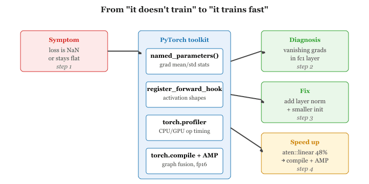
named_parameters() reveal whether activations are vanishing or exploding; forward hooks make shape mismatches visible; torch.profiler identifies which op (here aten::linear at 48% of CPU time) is the bottleneck; then torch.compile and AMP turn the diagnosis into wall-clock speed.0.4.1 Debugging: Hooks, Gradient Inspection, and Profiling
PyTorch hooks are the most powerful debugging feature almost nobody uses on their first project. They were originally added so researchers could implement custom backward passes for exotic gradient tricks, and ended up becoming the foundation for activation patching in modern interpretability work years later.
When your model does not train, you need tools to look inside. PyTorch provides several mechanisms for introspection.
0.4.1.1 Inspecting Gradients
After a backward pass, you can iterate over named parameters to check gradient statistics for signs of vanishing or exploding gradients.
# Check gradients after a backward pass
for name, param in model.named_parameters():
    if param.grad is not None:
        print(f"{name:20s} grad mean={param.grad.mean():.6f} "
f"std={param.grad.std():.6f}")0.4.1.2 Forward and Backward Hooks
Hooks let you inspect (or modify) data flowing through a module without changing its code. This is invaluable for debugging and later for techniques like activation patching in interpretability research.
import torch
# Register a forward hook that prints the output shape
def print_shape_hook(module, input, output):
    print(f"{module.__class__.__name__:15s} output shape: {output.shape}")
    hooks = []
    for name, layer in model.named_children():
        h = layer.register_forward_hook(print_shape_hook)
        hooks.append(h)
        # Run one forward pass to see shapes
        dummy = torch.randn(1, 784).to(device)
        _ = model(dummy)
        # Clean up hooks when done
        for h in hooks:
            h.remove()
0.4.1.3 Profiling with torch.profiler
The built-in profiler measures CPU and GPU time per operation, helping you identify performance bottlenecks.
# Profile a few training batches with torch.profiler to identify
# which operations (linear, cross_entropy, relu) consume the most CPU time.
from torch.profiler import profile, ProfilerActivity

# Profile execution to find performance bottlenecks
with profile(activities=[ProfilerActivity.CPU], record_shapes=True) as prof:
    for i, (images, labels) in enumerate(train_loader):
        images = images.view(images.size(0), -1)
        outputs = model(images)
        loss = criterion(outputs, labels)
        # Compute gradients via backpropagation
        loss.backward()
        if i >= 4:
            break

print(prof.key_averages().table(sort_by="cpu_time_total", row_limit=5))Profiling reveals where time is actually spent. In small models, data loading often dominates. In larger models, matrix multiplications dominate. Knowing this guides your optimization effort: increase num_workers for data-bound training, or use mixed precision for compute-bound training.
0.4.2 Common Mistakes and How to Fix Them
| Symptom | Cause | Fix |
|---|---|---|
RuntimeError: mat1 and mat2 shapes cannot be multiplied |
Input tensor shape does not match the layer's expected input dimension | Print shapes with print(x.shape) before each layer; ensure you flatten or reshape correctly |
Loss is nan after a few steps |
Learning rate is too high, or numerical overflow | Lower the learning rate; add gradient clipping with torch.nn.utils.clip_grad_norm_ |
| Loss never decreases | Forgot optimizer.zero_grad() or wrong loss function |
Verify the training loop skeleton; try overfitting on a single batch first |
Expected all tensors to be on the same device |
Model is on GPU but data is on CPU (or vice versa) | Call .to(device) on both model and data |
| Validation accuracy worse than training | Forgot model.eval() or torch.no_grad() |
Always wrap evaluation in model.eval() and with torch.no_grad(): |
Let us put everything together. In this lab you will build a fully connected neural network that classifies FashionMNIST images into 10 categories (T-shirt, Trouser, Pullover, Dress, Coat, Sandal, Shirt, Sneaker, Bag, Ankle boot). The complete script below is copy-pasteable and runnable.
#!/usr/bin/env python3
"""Lab 0.3: FashionMNIST Classifier in PyTorch (from scratch)."""

import torch
import torch.nn as nn
import torch.optim as optim
from torch.utils.data import DataLoader
from torchvision import datasets, transforms

# -- Hyperparameters ------------------------------------------
BATCH_SIZE = 64
LEARNING_RATE = 1e-3
NUM_EPOCHS = 10
HIDDEN_DIM = 256

# -- Device ---------------------------------------------------
device = torch.device("cuda" if torch.cuda.is_available() else "cpu")
print(f"Training on: {device}")

# -- Data -----------------------------------------------------
transform = transforms.Compose([
    transforms.ToTensor(),
    transforms.Normalize((0.2860,), (0.3530,)),
    ])

train_data = datasets.FashionMNIST("./data", train=True, download=True, transform=transform)
test_data = datasets.FashionMNIST("./data", train=False, download=True, transform=transform)

train_loader = DataLoader(train_data, batch_size=BATCH_SIZE, shuffle=True)
test_loader = DataLoader(test_data, batch_size=BATCH_SIZE, shuffle=False)

# -- Model ----------------------------------------------------
class FashionClassifier(nn.Module):
    def __init__(self, hidden_dim):
        super().__init__()
        self.net = nn.Sequential(
            nn.Flatten(), # (B,1,28,28) -> (B,784)
            nn.Linear(784, hidden_dim),
            nn.ReLU(),
            nn.Dropout(0.2),
            nn.Linear(hidden_dim, hidden_dim),
            nn.ReLU(),
            nn.Dropout(0.2),
            nn.Linear(hidden_dim, 10),
            )

    def forward(self, x):
        return self.net(x)

        model = FashionClassifier(HIDDEN_DIM).to(device)
        print(model)
        print(f"Parameters: {sum(p.numel() for p in model.parameters()):,}")

        # -- Loss and Optimizer ---------------------------------------
        criterion = nn.CrossEntropyLoss()
        optimizer = optim.Adam(model.parameters(), lr=LEARNING_RATE)

        # -- Training -------------------------------------------------
    def train_one_epoch(model, loader, criterion, optimizer, device):
        model.train()
        total_loss, correct, total = 0.0, 0, 0

        for images, labels in loader:
            images, labels = images.to(device), labels.to(device)

            optimizer.zero_grad()
            outputs = model(images)
            loss = criterion(outputs, labels)
            loss.backward()
            optimizer.step()

            total_loss += loss.item() * labels.size(0)
            correct += (outputs.argmax(1) == labels).sum().item()
            total += labels.size(0)

            return total_loss / total, correct / total

            # -- Evaluation -----------------------------------------------
def evaluate(model, loader, criterion, device):
    model.eval()
    total_loss, correct, total = 0.0, 0, 0

    with torch.no_grad():
        for images, labels in loader:
            images, labels = images.to(device), labels.to(device)
            outputs = model(images)
            loss = criterion(outputs, labels)

            total_loss += loss.item() * labels.size(0)
            correct += (outputs.argmax(1) == labels).sum().item()
            total += labels.size(0)

            return total_loss / total, correct / total

            # -- Run ------------------------------------------------------
            for epoch in range(NUM_EPOCHS):
                train_loss, train_acc = train_one_epoch(model, train_loader, criterion, optimizer, device)
                test_loss, test_acc = evaluate(model, test_loader, criterion, device)

                print(f"Epoch {epoch+1:2d}/{NUM_EPOCHS} "
                    f"Train Loss: {train_loss:.4f} Acc: {train_acc:.4f} "
                    f"Test Loss: {test_loss:.4f} Acc: {test_acc:.4f}")

                # -- Save -----------------------------------------------------
                torch.save({
                    "model_state_dict": model.state_dict(),
                    "optimizer_state_dict": optimizer.state_dict(),
                    "test_acc": test_acc,
                    }, "fashion_classifier_checkpoint.pth")
print(f"\nModel saved. Final test accuracy: {test_acc:.4f}")0.3.9.1 Lab Discussion
Let us dissect the key design decisions:
- Flatten layer: FashionMNIST images arrive as
(B, 1, 28, 28)tensors. Usingnn.Flatten()inside the model (rather than.view()outside) keeps the reshaping logic self-contained. - Dropout(0.2): Randomly zeroes 20% of activations during training. This regularizes the network and helps close the gap between train and test accuracy.
- Adam optimizer: Adapts the learning rate per parameter. A solid default for most problems; you rarely need to tune its internals.
- Separate train/eval functions: Keeping training and evaluation as standalone functions makes the code reusable. You will use this same skeleton for transformer models.
0.3.9.2 Exercises for Further Practice
- Overfit a single batch: Take one batch from the train loader and train on it for 100 steps. Can you drive the loss to zero? If yes, your model and training loop are correct. If no, you have a bug.
- Add a learning rate scheduler: Use
torch.optim.lr_scheduler.StepLRto decay the learning rate by 0.1 every 5 epochs. Does test accuracy improve? - Switch to a CNN: Replace the fully connected layers with convolutional layers (
nn.Conv2d,nn.MaxPool2d). You should be able to reach over 90% test accuracy. - Add gradient clipping: Insert
torch.nn.utils.clip_grad_norm_(model.parameters(), max_norm=1.0)beforeoptimizer.step(). Monitor the gradient norms before and after clipping.
0.4.3 Modern PyTorch: Performance and Scale
The training loop and model patterns covered so far are the foundation of every PyTorch project. However, modern deep learning, particularly LLM training and inference, demands tools that go beyond the basics. PyTorch 2.x introduced a compiler, and the ecosystem provides built-in support for mixed precision and distributed training. This section covers the three most important performance tools you will encounter in practice.
0.4.3.1 torch.compile and PyTorch 2.x
Starting with PyTorch 2.0, torch.compile transforms your eager-mode model into an
optimized graph that runs significantly faster. Under the hood, it uses TorchDynamo
to capture the computation graph from Python bytecode, then passes that graph to the
TorchInductor compiler backend, which generates optimized Triton (GPU) or C++/OpenMP
(CPU) kernels. The key insight is that you do not need to change your model code at all; you
simply wrap it with torch.compile() and let the compiler handle fusion, memory
planning, and kernel selection.
torch.compile offers three compilation modes, each trading compile time for runtime speed:
| Mode | Compile Time | Runtime Speed | Best For |
|---|---|---|---|
default | Fast | Good speedup | General use, quick iteration |
reduce-overhead | Moderate | Better (reduces CPU overhead) | Small batches, inference servers |
max-autotune | Slow (benchmarks many kernels) | Best possible | Production training, final deployment |
A few common pitfalls to watch for: (1) the first call triggers compilation, so you will see a
one-time latency spike; (2) data-dependent control flow (e.g., if x.sum() > 0)
causes "graph breaks" that reduce optimization opportunities; and (3) not all custom CUDA
extensions are supported yet. When in doubt, start with default mode and profile.
# torch.compile: wrap a model for optimized GPU kernel generation.
# The first call triggers compilation; subsequent calls run faster.
import torch

# Define a simple model
model = MyTransformerBlock(d_model=512, n_heads=8).cuda()

# Without torch.compile: standard eager execution
output_eager = model(input_tensor)

# With torch.compile: optimized execution
compiled_model = torch.compile(model, mode="reduce-overhead")

# First call triggers compilation (slow), subsequent calls are fast
output_compiled = compiled_model(input_tensor)

# In benchmarks, expect 1.3x to 2x speedup on Transformer blockstorch.compile in reduce-overhead mode. The compiled model produces identical output but runs 1.3x to 2x faster after the one-time compilation cost.Advanced torch.compile: Dynamic Shapes, Fullgraph Mode, and Debugging
Getting the most out of torch.compile in production requires understanding three
additional concepts beyond the basic wrapper. First, dynamic shapes: by default,
the compiler assumes fixed input shapes and triggers a full recompilation whenever the shape
changes. For NLP workloads where sequence lengths vary across batches, this causes repeated
compilations that negate any speedup. Setting dynamic=True tells the compiler to
generate shape-generic kernels that work across a range of input sizes, at the cost of slightly
less aggressive optimization for any single shape. In Transformer training with variable-length
sequences, dynamic=True is almost always the right choice.
Second, fullgraph mode: the fullgraph=True option tells the compiler
to capture the entire model as a single graph, which enables global optimizations but will raise
an error if any graph break occurs. This is useful for validating that your model is fully
compilable before deploying to production. If graph breaks are present, the compiler silently
falls back to partial compilation, which may deliver only modest speedups. Running with
fullgraph=True during development ensures you catch and eliminate graph breaks early.
Third, debugging and profiling: the torch._dynamo module exposes
configuration flags that help you understand what the compiler is doing. Setting
torch._dynamo.config.verbose = True logs every graph break with a traceback,
making it straightforward to identify problematic code patterns. The
torch.utils.benchmark module provides a clean way to compare eager and compiled
execution times with statistically meaningful measurements.
# Strict mode: fails if any graph break is detected
compiled_strict = torch.compile(model, fullgraph=True)

# Dynamic shapes: avoid recompilation when input sizes change
compiled_dynamic = torch.compile(model, dynamic=True)

# Combine max-autotune with fullgraph for production
compiled_prod = torch.compile(
 model,
 mode="max-autotune",
 fullgraph=True,
 dynamic=True,
)

# Debugging: see what the compiler is doing
import torch._dynamo
torch._dynamo.config.verbose = True # Log graph breaks with tracebacks
torch._dynamo.config.suppress_errors = False # Fail loudly on issues

# Profile compiled vs. eager to measure actual speedup
import torch.utils.benchmark as bench

timer_eager = bench.Timer(
 stmt="model(x)",
 globals={"model": model, "x": input_tensor},
)
timer_compiled = bench.Timer(
 stmt="compiled_model(x)",
 globals={"compiled_model": compiled_prod, "x": input_tensor},
)

print(f"Eager: {timer_eager.timeit(100).mean * 1000:.2f} ms")
print(f"Compiled: {timer_compiled.timeit(100).mean * 1000:.2f} ms")torch.export: Deployment Beyond Python
PyTorch 2.x also introduced torch.export, which captures a model as a clean,
self-contained graph representation suitable for deployment outside of Python. While
torch.compile accelerates training and eager-mode inference,
torch.export targets production deployment scenarios: shipping a model to a mobile
device, embedding it in a C++ application, or converting it to a format consumed by a
purpose-built serving stack. The exported graph can be lowered to backends like ExecuTorch
(for edge and mobile devices) or AOTInductor (for server deployment without the Python
runtime overhead).
import torch
# torch.export: capture a deployment-ready graph
from torch.export import export
# Define example inputs for tracing
example_input = torch.randn(1, 128, 512).cuda()
# Export the model (captures the full graph)
exported = export(model, (example_input,))
# The exported program can be serialized and loaded without Python
torch.export.save(exported, "model_exported.pt2")
# For server deployment with AOTInductor (generates a .so library)
# torch._inductor.aot_compile(model, (example_input,))FSDP2 and torch.compile. PyTorch 2.4 and later includes a rewritten Fully Sharded Data Parallel implementation (commonly called FSDP2 or fully_shard in the torch.distributed namespace) designed to compose cleanly with torch.compile. The original FSDP relied on runtime hooks that caused graph breaks, limiting compilation benefits. FSDP2 integrates sharding logic directly into the compiler graph, enabling end-to-end optimization of distributed training. If you are training large models across multiple GPUs and want both sharding and compilation, FSDP2 is the recommended path.
Combining torch.compile with Mixed Precision
In practice, torch.compile and mixed precision are used together rather than
in isolation. The compiler is aware of autocast regions and can fuse operations
across precision boundaries, generating kernels that perform the cast and the computation in a
single step. This combination typically yields the best results: mixed precision reduces memory
traffic and enables Tensor Core utilization, while the compiler eliminates kernel launch overhead
and fuses adjacent operations. The following example shows the recommended production pattern
that combines both techniques.
# Combine torch.compile (max-autotune) with BF16 autocast.
# The compiler fuses cast and compute into single GPU kernels.
import torch
from torch.amp import autocast

# Compile the model first
model = MyTransformerBlock(d_model=512, n_heads=8).cuda()
compiled_model = torch.compile(model, mode="max-autotune", dynamic=True)

optimizer = torch.optim.AdamW(compiled_model.parameters(), lr=3e-4)

for batch_x, batch_y in train_loader:
    batch_x, batch_y = batch_x.cuda(), batch_y.cuda()
    optimizer.zero_grad()

    # BF16 autocast inside the compiled model: the compiler fuses casts
    with autocast(device_type="cuda", dtype=torch.bfloat16):
        output = compiled_model(batch_x)
        loss = criterion(output, batch_y)

        loss.backward()
        optimizer.step()

        # On Ampere+ GPUs, this pattern typically yields 2x to 3x throughput
# improvement over eager FP32 execution.0.4.3.2 Mixed Precision Training with torch.amp
Modern GPUs have specialized hardware (Tensor Cores) that operate much faster on 16-bit floating-point numbers than on 32-bit. Mixed precision training uses 16-bit for most operations (forward pass, backward pass) while keeping a 32-bit master copy of the weights for the optimizer update. This roughly halves memory usage and can double training throughput.
PyTorch provides torch.amp (Automatic Mixed Precision) with two components:
torch.amp.autocast automatically selects the right precision for each operation
(matmuls in FP16/BF16, reductions in FP32), and torch.amp.GradScaler prevents
underflow by scaling the loss before the backward pass and unscaling gradients before the
optimizer step. On Ampere GPUs (A100, RTX 3090) and newer, BF16 (bfloat16) is
preferred over FP16 because it has the same exponent range as FP32, which eliminates most
overflow/underflow issues and makes GradScaler unnecessary.
# Mixed-precision training with GradScaler (FP16) and autocast.
# GradScaler prevents gradient underflow; skip it when using BF16.
import torch
from torch.amp import autocast, GradScaler

model = MyModel().cuda()
optimizer = torch.optim.AdamW(model.parameters(), lr=3e-4)
scaler = GradScaler() # Only needed for FP16; skip for BF16

for epoch in range(num_epochs):
    for batch_x, batch_y in train_loader:
        batch_x, batch_y = batch_x.cuda(), batch_y.cuda()
        optimizer.zero_grad()

        # Forward pass in mixed precision
        with autocast(device_type="cuda", dtype=torch.float16):
            output = model(batch_x)
            loss = criterion(output, batch_y)

            # Backward pass with gradient scaling
            scaler.scale(loss).backward()
            scaler.step(optimizer)
            scaler.update()

            # For BF16 (preferred on Ampere+ GPUs), simply use:
                # with autocast(device_type="cuda", dtype=torch.bfloat16):
                    # output = model(batch_x)
                    # loss = criterion(output, batch_y)
                    # loss.backward() # No scaler needed
# optimizer.step()0.4.3.3 Distributed Data Parallel (DDP)
When a single GPU is not enough, torch.nn.parallel.DistributedDataParallel (DDP) is
the standard way to scale training across multiple GPUs (or multiple machines). DDP replicates
the model on each GPU, splits each batch across the replicas, and synchronizes gradients with an
all-reduce operation after each backward pass. Because each GPU processes a different slice of
the data, the effective batch size scales linearly with the number of GPUs.
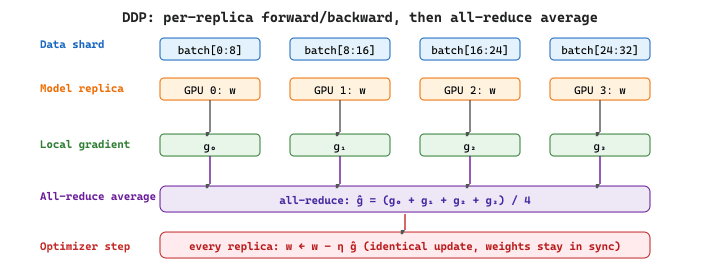
Concretely, DDP estimates the gradient of the per-example loss as the average over the global batch of size $B = K \cdot b$, where $K$ is the number of replicas and $b$ the per-GPU micro-batch:
$$ g \;=\; \frac{1}{B} \sum_{i=1}^{B} \nabla_{\theta} \ell(x_i; \theta) \;=\; \frac{1}{K} \sum_{k=1}^{K} \underbrace{\frac{1}{b} \sum_{i \in \text{shard}_k} \nabla_{\theta} \ell(x_i; \theta)}_{g_k\, \text{computed on GPU}\, k} $$
That second equality is exactly what the all-reduce computes: each GPU first averages over its own shard locally, then the ring all-reduce averages the $g_k$ across replicas. The result is mathematically identical to running a single GPU at the full batch size $B$, which is why the linear scaling rule (multiply the learning rate by $K$) usually holds.
DDP is preferred over the older DataParallel because it avoids the GIL bottleneck
and overlaps communication with computation. Setting it up requires initializing a process group
and wrapping your model, but the training loop itself remains almost identical to the single-GPU
version. For LLM training at larger scales, you will encounter FSDP (Fully Sharded Data
Parallel), which shards both parameters and gradients across GPUs. We will revisit distributed
training in Chapter 06 when we discuss pretraining.
import os
# Distributed Data Parallel: initialize a process group, wrap the model,
# and train with automatic gradient synchronization across GPUs.
import torch
import torch.distributed as dist
from torch.nn.parallel import DistributedDataParallel as DDP
# Initialize the process group (one process per GPU)
dist.init_process_group(backend="nccl")
local_rank = int(os.environ["LOCAL_RANK"])
torch.cuda.set_device(local_rank)
# Create model and wrap with DDP
model = MyModel().cuda(local_rank)
model = DDP(model, device_ids=[local_rank])
# Training loop is the same as single-GPU
for batch_x, batch_y in train_loader:
    optimizer.zero_grad()
    output = model(batch_x.cuda(local_rank))
    loss = criterion(output, batch_y.cuda(local_rank))
    loss.backward() # DDP handles gradient sync automatically
    optimizer.step()
    # Launch with: torchrun --nproc_per_node=4 train.py
0.4.3.4 DDP in Practice: What Happens Under the Hood
Understanding DDP's mechanics helps you debug distributed training issues and make informed choices
about scaling. When you wrap a model with DistributedDataParallel, three things happen
at initialization: (1) the model parameters are broadcast from rank 0 to all other processes, ensuring
every GPU starts with identical weights; (2) DDP registers backward hooks on every parameter, which
trigger gradient synchronization automatically; and (3) parameters are grouped into "buckets" for
communication efficiency, so that all-reduce operations overlap with backward computation.
The bucket-based overlap is critical for performance. Rather than waiting until all gradients are
computed and then performing a single all-reduce, DDP starts synchronizing the gradients of later
layers (which finish their backward pass first) while earlier layers are still computing. This
overlap means that for well-balanced models, communication is almost entirely hidden behind computation.
You can control bucket size with the bucket_cap_mb parameter (default: 25 MB).
A few practical details matter when using DDP:
- DistributedSampler: Each GPU must see a different subset of the data. Use
torch.utils.data.distributed.DistributedSamplerwith your DataLoader to ensure non-overlapping splits. Remember to callsampler.set_epoch(epoch)at the start of each epoch so that shuffling differs across epochs. - Batch size scaling: The effective batch size is
per_gpu_batch_size * num_gpus. If you increase from 1 GPU to 8 GPUs, the effective batch size grows 8x. You may need to adjust the learning rate accordingly (linear scaling rule: multiply learning rate by the same factor). - Saving checkpoints: Only save from rank 0 to avoid duplicate writes. Guard your save
logic with
if dist.get_rank() == 0. - Launching: Use
torchrun(ortorch.distributed.launch) to spawn one process per GPU. For multi-node training, you also need to set--nnodes,--node_rank, and--master_addr.
from torch.utils.data import DataLoader
import torch
# Complete DDP training setup with DistributedSampler
from torch.utils.data.distributed import DistributedSampler
sampler = DistributedSampler(train_dataset, shuffle=True)
train_loader = DataLoader(train_dataset, batch_size=32, sampler=sampler)
for epoch in range(num_epochs):
    sampler.set_epoch(epoch) # Ensure different shuffling each epoch
    for batch_x, batch_y in train_loader:
        optimizer.zero_grad()
        output = model(batch_x.cuda(local_rank))
        loss = criterion(output, batch_y.cuda(local_rank))
        loss.backward()
        optimizer.step()
        # Save only from rank 0
        if dist.get_rank() == 0:
            torch.save(model.module.state_dict(), f"checkpoint_epoch_{epoch}.pt")
Note the use of model.module.state_dict() rather than model.state_dict()
when saving. The DDP wrapper adds a .module attribute that references the original model.
Saving through .module produces a state dict compatible with non-DDP loading, which is
almost always what you want.
Train a 350M-parameter encoder with per-GPU batch $b = 32$ on four 80 GB A100s connected by NVLink. Effective global batch is $B = 4 \times 32 = 128$. Following the linear scaling rule, the learning rate moves from a single-GPU baseline of $1 \cdot 10^{-4}$ to $4 \cdot 10^{-4}$.
Each backward pass produces roughly $350\text{M} \times 4\,\text{bytes} \approx 1.4$ GB of FP32 gradients per replica. NVLink delivers about 600 GB/s, so a naive all-reduce would take $1.4 / 600 \approx 2.3$ ms; the ring algorithm's $2(K-1)/K$ factor pushes that to roughly 3.5 ms. A single optimizer step on the 350M model takes about 80 ms of pure compute, so the gradient sync hides almost completely behind the still-running backward pass via DDP's bucket scheduling. Wall-clock speedup over a single GPU lands near $3.7\times$ rather than the ideal $4\times$, with the gap explained almost entirely by the residual all-reduce that does not overlap.
DDP works well when the entire model, its gradients, and the optimizer states fit in a single GPU's memory. For a 7B parameter model with AdamW in FP32, that total is roughly 112 GB, which exceeds even an 80 GB A100. At that point, you need FSDP (Fully Sharded Data Parallel) or DeepSpeed ZeRO, which shard parameters and optimizer states across GPUs. We cover these techniques in detail in Section 6.6.
At the top of every training script, set torch.manual_seed(42), random.seed(42), and np.random.seed(42). Reproducibility saves hours of debugging when results change between runs for no obvious reason.
PyTorch continues to evolve rapidly. PyTorch 2.x introduced torch.compile, which automatically generates optimized GPU kernels through graph capture and code generation. The ecosystem now includes torchtune for LLM fine-tuning, torchchat for local inference, and tight integration with Hugging Face Transformers and Accelerate for distributed training. Meanwhile, JAX/Flax remains the primary alternative for large-scale training at Google.
- Tensors are the atomic data structure. Master creation, reshaping, indexing, and device management before anything else.
- Autograd builds a computational graph dynamically. Calling
.backward()walks the graph in reverse to compute gradients. Always remember to zero gradients between iterations. - nn.Module organizes your model. Define layers in
__init__, wire them inforward, and call the model (not.forward()directly) to benefit from hooks and other machinery. - DataLoader handles batching, shuffling, and parallel loading. Pair it with
Datasetfor standard or custom data. - The training loop follows a fixed rhythm: zero gradients, forward, loss, backward, step. Every neural network training (from this classifier to GPT) follows this pattern.
- Checkpointing saves both model and optimizer state so you can resume training after interruptions. Use
state_dictfor portability. - Debugging tools (hooks, gradient inspection, profiler) are not luxuries. Use them early and often. A few minutes of profiling can save hours of guessing.
- Start simple. Overfit a single batch. Then scale to the full dataset. Then tune. This progression catches bugs at the cheapest possible stage.
1. You create two tensors: a = torch.randn(3, 4) on CPU and b = torch.randn(3, 4).cuda() on GPU. What happens when you compute a + b, and how do you fix it?
Show Answer
RuntimeError: Expected all tensors to be on the same device. Tensor operations require all operands to live on the same device; the framework will not silently copy across the CPU/GPU boundary because that would mask serious performance problems. The fix is to move one tensor to match the other, typically a = a.to(b.device) (or a = a.cuda()). In real training loops you set device = torch.device("cuda" if torch.cuda.is_available() else "cpu") once at the top and call .to(device) on every tensor and every model.2. After calling loss.backward() twice in a row without optimizer.zero_grad(), what value does each parameter's .grad hold relative to the true gradient? Why is this behavior the default?
Show Answer
.grad holds the SUM of the two backward-pass gradients, not the most recent one. PyTorch accumulates gradients by design so that you can split a logical batch across several smaller forward/backward passes (gradient accumulation for low-VRAM training) by calling backward() multiple times before stepping. The cost of that flexibility is that every standard training loop must explicitly call optimizer.zero_grad() (or set the gradients to None via set_to_none=True, slightly faster) before each new backward pass.3. Explain the difference between torch.compile(model) and torch.export(model, (example_input,)). When would you choose each one?
Show Answer
torch.compile applies JIT optimization in-process, keeping the Python runtime in the loop. It traces the model on first call, lowers the captured graph through TorchInductor to fused kernels, and falls back to eager Python whenever it encounters something it cannot capture (data-dependent control flow, dynamic shapes, etc.). Use it when you want speedups during research or training without changing your deployment story. torch.export produces a serializable graph (ExportedProgram) with no Python dependency. It is stricter: data-dependent control flow has to be expressed as graph operations, dynamic shapes need explicit specification, and the result is a portable artifact you can run with ExecuTorch on mobile, deploy with AOT compilation, or load on a server with no Python. Choose torch.compile for in-process performance; choose torch.export when you need a static, portable graph.Exercises
You have a tensor of shape (B=32, T=128, D=512). (a) After a linear layer with output dim 1024, what shape do you get? (b) After mean-pooling over the T dimension, what shape? (c) After an attention over the T dimension with no head dimension explicit, what shape?
Answer Sketch
(a) Linear layer applies to the last dim: (32, 128, 1024). The first two dims pass through unchanged. (b) Mean-pool over dim T: (32, 512). (c) Attention preserves the shape: (32, 128, 512). Attention is a sequence-to-sequence operation where each position's output is a weighted average of all positions; the time dimension is preserved. The general rule for shape-tracking: identify which dim each operation acts on (last dim for linear, specified dim for pool/attention, batch dim for batched matmul) and the others pass through.
Predict whether autograd will compute gradients in each case: (a) x = torch.randn(3, 4); y = x.mean(); y.backward(); (b) the same with x = torch.randn(3, 4, requires_grad=True); (c) the same wrapped in with torch.no_grad():. State the design intent of each behavior.
Answer Sketch
(a) Errors: y has no grad_fn because x has requires_grad=False by default, so autograd has nothing to differentiate. (b) Works: x.grad is populated with shape (3, 4), each entry 1/12 (the partial derivative of mean over 12 elements). (c) Errors / no-op: no_grad disables autograd tracking, so y has no grad_fn even with requires_grad=True. Design intent: (a) avoid wasting memory on graphs you didn't ask for; (b) explicit opt-in to differentiation for trainable parameters; (c) explicit opt-out for inference and validation paths to save memory and speed up forward passes by ~20-30%.
Write a 12-line PyTorch training loop for a simple regression problem: model with one linear layer, MSE loss, SGD, 100 epochs, no DataLoader (use a fixed (X, y) pair). State the one line you would add for production-grade training.
Answer Sketch
import torch; from torch import nn
X = torch.randn(100, 5); y = X @ torch.randn(5, 1) + 0.1 * torch.randn(100, 1)
model = nn.Linear(5, 1)
opt = torch.optim.SGD(model.parameters(), lr=0.01)
loss_fn = nn.MSELoss()
for epoch in range(100):
  opt.zero_grad()
  pred = model(X)
  loss = loss_fn(pred, y)
  loss.backward()
  opt.step()
if epoch % 10 == 0: print(f"epoch {epoch} loss {loss.item():.4f}")The one production line: gradient clipping. Add torch.nn.utils.clip_grad_norm_(model.parameters(), 1.0) between backward() and step(). This prevents loss spikes from individual outlier batches and is essentially mandatory for any non-toy training run, especially with Adam or AdamW.
List four PyTorch bugs that silently produce wrong results (no exception raised), with one diagnostic for each.
Answer Sketch
(1) Forgot to call opt.zero_grad(): gradients accumulate across batches; loss decreases erratically. Diagnostic: log gradient norms; you'll see them grow over time. (2) Calling .eval() on the model instead of .train() during training: dropout and batchnorm behave wrong; train loss is suspiciously low. Diagnostic: sanity-check by toggling and observing batchnorm running stats. (3) Mixing tensors on CPU and GPU: silent slowdowns, sometimes silent NaN propagation when using older versions. Diagnostic: assert all parameter and input tensors share .device. (4) Loss using .item() in the graph: detaching the loss before backward; gradient never updates. Diagnostic: print loss.requires_grad before backward(); should be True. The general principle: PyTorch is permissive on purpose, so explicit assertions in your training loop catch these bugs in seconds.
What's Next?
In the next section, Section 0.5: Reinforcement Learning Foundations, we introduce reinforcement learning foundations, which will become essential when we study RLHF and alignment techniques later in the book.