I trained a Word2Vec model and then a BERT model on the same corpus. Word2Vec finished before lunch. BERT finished my electricity budget.
Lexica, Carbon-Aware AI Agent
This section continues from Section 1.4, which walked through the polysemy problem, ELMo, contextual embeddings in code, and what changed when Transformers replaced LSTMs. Here we put it all into practice: a hands-on lab comparing static and contextual embeddings, a step-by-step walk through BERT's pretraining recipe (MLM + NSP), and exercises that consolidate the static-to-contextual story.
Prerequisites
This section continues from Section 1.4. Familiarity with ELMo, the polysemy problem, static vs contextual embeddings, and the basic biLSTM architecture covered there is assumed.
The 15% masking rate in BERT's MLM objective was not derived from theory. The original authors tried a few values, noticed 15% worked, and moved on. Years of follow-up research, RoBERTa, SpanBERT, ELECTRA, partially exists to relitigate that arbitrary choice. The lesson: in pretraining, hyperparameters that look like sacred constants are often the first value someone tried on a Tuesday.
Having traced the representation journey from static to contextual in Section 1.4, we now consolidate with a lab, the canonical BERT pretraining recipe, and exercises that test the static-vs-contextual distinction.
- A text preprocessing pipeline in both NLTK and spaCy
- Bag-of-Words and TF-IDF vectorizers with sklearn
- A Word2Vec model trained from scratch with Gensim
- Cosine similarity computations and word analogy queries
- A FastText model that handles out-of-vocabulary words
- GloVe vectors loaded and compared with Word2Vec
- A similarity heatmap and t-SNE visualization
- Contextual embeddings extracted from BERT, proving that "bank" gets different vectors in different contexts
You now have hands-on experience with every major text representation technique from the past 30 years. Not bad for one chapter.
Show Answer
Show Answer
Show Answer
Lab: Word2Vec and Contextual Embeddings
Objective
Train a Word2Vec model from scratch with gensim, visualize word relationships using t-SNE, then compare static embeddings with contextual embeddings from a pretrained transformer to see how context changes word representations.
Skills Practiced
- Training Word2Vec (Skip-gram and CBOW) using gensim
- Querying word analogies and nearest neighbors in embedding space
- Visualizing high-dimensional embeddings with t-SNE
- Extracting contextual embeddings from a pretrained model
- Comparing static vs. contextual representations for polysemous words
Setup
Install the required packages for this lab.
pip install gensim matplotlib scikit-learn transformers torch numpySteps
Step 1: Train Word2Vec on a sample corpus
Use gensim to train a Skip-gram Word2Vec model. Even on a small corpus, the model learns meaningful word relationships through the distributional hypothesis.
from gensim.models import Word2Vec
# Sample corpus (in practice, use a larger dataset)
sentences = [
    ["the", "king", "rules", "the", "kingdom"],
    ["the", "queen", "rules", "the", "kingdom"],
    ["a", "prince", "is", "the", "son", "of", "a", "king"],
    ["a", "princess", "is", "the", "daughter", "of", "a", "king"],
    ["the", "man", "works", "in", "the", "city"],
    ["the", "woman", "works", "in", "the", "city"],
    ["a", "boy", "plays", "in", "the", "park"],
    ["a", "girl", "plays", "in", "the", "park"],
    ["the", "dog", "runs", "in", "the", "park"],
    ["the", "cat", "sleeps", "on", "the", "couch"],
    ] * 100 # Repeat for better training
model = Word2Vec(sentences, vector_size=50, window=3,
    min_count=1, sg=1, epochs=50)
# Query nearest neighbors
for word in ["king", "queen", "man"]:
    neighbors = model.wv.most_similar(word, topn=3)
print(f"{word}: {[(w, f'{s:.2f}') for w, s in neighbors]}")Step 2: Visualize embeddings with t-SNE
Project the 50-dimensional word vectors down to 2D for visualization. Words with similar meanings should cluster together.
import matplotlib.pyplot as plt
from sklearn.manifold import TSNE
import numpy as np
words = list(model.wv.key_to_index.keys())
vectors = np.array([model.wv[w] for w in words])
tsne = TSNE(n_components=2, random_state=42, perplexity=min(5, len(words) - 1))
coords = tsne.fit_transform(vectors)
fig, ax = plt.subplots(figsize=(10, 8))
ax.scatter(coords[:, 0], coords[:, 1], s=40, alpha=0.6)
for i, word in enumerate(words):
    ax.annotate(word, (coords[i, 0], coords[i, 1]),
        fontsize=9, ha="center", va="bottom")
    ax.set_title("Word2Vec Embeddings (t-SNE projection)")
    ax.grid(True, alpha=0.3)
    plt.tight_layout()
    plt.savefig("word2vec_tsne.png", dpi=150)
plt.show()Step 3: Compare static vs. contextual embeddings
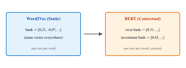
Use a pretrained transformer to show that "bank" gets different representations depending on context, unlike Word2Vec where it always maps to the same vector. This is the core insight from ELMo that this section covers.
from transformers import AutoTokenizer, AutoModel
import torch
import numpy as np
tokenizer = AutoTokenizer.from_pretrained("bert-base-uncased")
bert = AutoModel.from_pretrained("bert-base-uncased")
sentences = [
    "I deposited money at the bank",
    "We sat on the river bank",
    "The bank approved the loan",
    "Fish swim near the bank of the stream",
    ]
def get_word_embedding(sentence, target_word):
    """Extract BERT embedding for a target word in context."""
    inputs = tokenizer(sentence, return_tensors="pt")
    tokens = tokenizer.convert_ids_to_tokens(inputs["input_ids"][0])
    with torch.no_grad():
        outputs = bert(**inputs)
        # Find the target word's token index
        idx = next(i for i, t in enumerate(tokens) if target_word in t)
        return outputs.last_hidden_state[0, idx].numpy()
        # Get "bank" embeddings in each context
        embeddings = [get_word_embedding(s, "bank") for s in sentences]
        # Compute pairwise cosine similarity
        from numpy.linalg import norm
        print("Cosine similarity between 'bank' in different contexts:")
        for i in range(len(sentences)):
            for j in range(i + 1, len(sentences)):
                cos_sim = np.dot(embeddings[i], embeddings[j]) / (
                    norm(embeddings[i]) * norm(embeddings[j]))
                print(f" [{i}] vs [{j}]: {cos_sim:.3f}")
print(f" '{sentences[i]}' vs '{sentences[j]}'")Expected pattern
Financial sentences (0 and 2) should have higher cosine similarity with each other than with the river sentences (1 and 3). This confirms that BERT produces different representations for "bank" depending on context, unlike Word2Vec.
Step 4: Visualize contextual differences
Plot a heatmap of cosine similarities to see the clustering of financial vs. geographic senses.
import numpy as np
import matplotlib.pyplot as plt
from numpy.linalg import norm
n = len(embeddings)
sim_matrix = np.zeros((n, n))
for i in range(n):
    for j in range(n):
        sim_matrix[i, j] = np.dot(embeddings[i], embeddings[j]) / (
            norm(embeddings[i]) * norm(embeddings[j]))
        fig, ax = plt.subplots(figsize=(6, 5))
        im = ax.imshow(sim_matrix, cmap="RdYlGn", vmin=0.7, vmax=1.0)
        short_labels = ["money at bank", "river bank", "bank approved", "bank of stream"]
        ax.set_xticks(range(n))
        ax.set_xticklabels(short_labels, rotation=45, ha="right", fontsize=9)
        ax.set_yticks(range(n))
        ax.set_yticklabels(short_labels, fontsize=9)
        for i in range(n):
            for j in range(n):
                ax.text(j, i, f"{sim_matrix[i,j]:.2f}", ha="center", va="center", fontsize=10)
                ax.set_title("Contextual Similarity of 'bank' (BERT)")
                plt.colorbar(im, ax=ax, shrink=0.8)
                plt.tight_layout()
                plt.savefig("contextual_bank.png", dpi=150)
                plt.show()
Stretch Goals
- Try the same polysemy experiment with other ambiguous words like "bat," "crane," or "spring."
- Extract embeddings from different BERT layers and compare how the representations change from layer 1 (more syntactic) to layer 12 (more semantic).
- Train Word2Vec on a larger corpus (e.g., gensim's built-in text8 dataset) and test the classic king - man + woman = queen analogy.
- Context changes meaning. Unlike static embeddings, contextual embeddings produce different vectors for the same word in different sentences, solving the polysemy problem.
- ELMo pioneered the "pretrain then fine-tune" paradigm. A bidirectional LSTM is pretrained on a large corpus, then its internal representations are used as features for downstream tasks.
- Different layers capture different information. Lower ELMo layers encode syntax (part of speech, word order), while upper layers capture semantics (word sense, sentiment).
- ELMo's limitations motivated Transformers. Sequential processing limits parallelism and long-range dependencies, leading directly to the attention-based architecture covered in Chapter 04.
Exercises & Self-Check Questions
The conceptual questions test your understanding of the why behind each technique. Try answering them in your own words before moving on. The coding exercises are hands-on challenges you should run in a Jupyter notebook.
Conceptual Questions
- Representation evolution: In your own words, explain why the transition from sparse vectors (BoW) to dense vectors (Word2Vec) was such a big deal. What specific problems did it solve, and what new capabilities did it unlock?
- The distributional hypothesis: The phrase "you shall know a word by the company it keeps" is the foundation of Word2Vec. Can you think of cases where this assumption breaks down? (Hint: think about antonyms. "Hot" and "cold" appear in very similar contexts...)
- Static vs. contextual: Give three sentences where the word "play" means different things. Explain why Word2Vec would struggle with these but ELMo would handle them well.
- Why pretrain? ELMo was pretrained on a large corpus, then used for specific tasks. Why is this better than training a model from scratch for each task? What does the pretraining capture that task-specific training would miss?
- Trade-offs: A colleague argues "TF-IDF is obsolete; just use embeddings for everything." Give two scenarios where TF-IDF would actually be the better choice, and explain why.
Coding Exercises
- Preprocessing exploration: Take a paragraph from a news article. Run it through the preprocessing pipeline from Section 1.2. Then experiment: what happens if you do not remove stop words? What if you use stemming instead of lemmatization? How do the resulting BoW vectors differ?
- Analogy hunting: Using the pretrained
word2vec-google-news-300vectors, find 5 analogies that work well (beyond king/queen) and 3 that fail. Can you explain why the failures happen? - Similarity exploration: Pick 20 words from three different categories (e.g., sports, food, technology). Compute all pairwise cosine similarities. Do words within a category have higher similarity than cross-category pairs? Visualize the similarity matrix as a heatmap.
- Word2Vec from scratch (challenge): Implement the Skip-gram model with negative sampling in pure PyTorch (no Gensim). Train it on a small text corpus and verify that similar words end up with similar vectors. Compare your results with Gensim's output.
- Scaffolding hint: Your implementation will need four key components:
(1) a
SkipGramDatasetclass that generates (center, context, negative) tuples from your corpus; (2) twonn.Embeddinglayers, one for center words and one for context words; (3) a negative sampling loss function that maximizes the dot product for positive pairs and minimizes it for negative pairs (see the formula in Section 1.3); and (4) a training loop that iterates over batches, computes the loss, and callsoptimizer.step(). Start with a small vocabulary (a few hundred words) and short embedding dimension (50) to debug before scaling up.
Further Reading
| Topic | Paper / Resource | Why Read It |
|---|---|---|
| Word2Vec | Mikolov et al., "Efficient Estimation of Word Representations in Vector Space" (2013) | The original paper. Surprisingly short and readable. |
| GloVe | Pennington et al., "GloVe: Global Vectors for Word Representation" (2014) | Elegant math showing why co-occurrence ratios encode meaning. |
| FastText | Bojanowski et al., "Enriching Word Vectors with Subword Information" (2017) | The subword approach that later influenced BPE tokenizers. |
| ELMo | Peters et al., "Deep contextualized word representations" (2018) | The paper that proved contextual embeddings work on every task. |
| Word2Vec explained | Jay Alammar, "The Illustrated Word2Vec" | The best visual explanation of Word2Vec on the internet. |
| Embeddings theory | Levy & Goldberg, "Neural Word Embedding as Implicit Matrix Factorization" (2014) | The mathematical connection between Word2Vec and GloVe. |
You now understand how text becomes numbers: from sparse one-hot vectors to dense Word2Vec embeddings to contextual ELMo representations. But all these methods assumed words were already given to you. In Chapter 1: Tokenization and Subword Models, you will discover that the choice of how to split text into units is itself a critical design decision. BPE, WordPiece, and Unigram determine the atoms of the model's world, and those atoms affect everything from multilingual performance to arithmetic reasoning to API cost.
Exercises
For the sentence "I deposited the check at the bank by the river", state what (a) Word2Vec, (b) ELMo, and (c) BERT each produce for the word "bank", and explain how each progressively addresses the polysemy problem.
Answer Sketch
(a) Word2Vec: a single static vector for "bank" averaging the financial and river senses; identical regardless of sentence. (b) ELMo: a context-dependent vector formed by combining a forward and backward LSTM's hidden states at this position; different for "bank" in financial vs river contexts but produced from a shallow biLM. (c) BERT: a fully bidirectional transformer hidden state at the "bank" position; richer context integration via self-attention over the whole sentence and far higher representational capacity. The trajectory is "more context, more parameters, less polysemy"; modern LLM internal representations are the natural endpoint.
ELMo combines representations from multiple LSTM layers. For a downstream task, predict (a) which layer's representation is most useful for syntax tasks (POS, chunking), (b) which is most useful for semantics (NER, sentiment), and (c) why ELMo learns a per-task layer-mixing weight rather than picking one.
Answer Sketch
(a) Lower layers are most useful for syntax: closer to surface form, encoding morphology and POS-style information. (b) Higher layers are most useful for semantics: more abstracted, encoding word sense and entity-type information. (c) ELMo learns per-task layer weights because the optimal mix varies: a chunking task wants more lower-layer, a question-answering task wants more upper-layer. A learned weighted sum lets the same pretrained model serve all tasks without specialized re-training. This same insight drives modern probe-based analyses of Transformer layers (Chapter 11 Interpretability).
Sketch a 6-line snippet that uses Hugging Face transformers to extract the contextual BERT embedding for a specific token in a sentence. Show how the same token has different embeddings in two sentences.
Answer Sketch
import torch
from transformers import AutoTokenizer, AutoModel
tok = AutoTokenizer.from_pretrained("bert-base-uncased"); model = AutoModel.from_pretrained("bert-base-uncased")
def embed(sentence, target_word):
    enc = tok(sentence, return_tensors="pt")
    out = model(**enc).last_hidden_state[0]
    idx = enc.tokens().index(target_word)
    return out[idx]
v1 = embed("I deposited money at the bank.", "bank")
v2 = embed("We sat by the river bank.", "bank")
print(torch.cosine_similarity(v1, v2, dim=0)) # roughly 0.5-0.7, not 1.0
The output is far below 1.0, demonstrating that BERT produces genuinely different vectors for the same surface token in different contexts. Word2Vec would return 1.0 (same vector). This single experiment is the cleanest empirical demonstration of why contextual embeddings replaced static ones.
ELMo was the first widely-used contextual embedding model in 2018; by 2019 BERT had largely replaced it. Identify three architectural or workflow reasons ELMo lost, beyond just "BERT is bigger." For each, explain why the same reason applies to current LLMs vs older RNN-based systems.
Answer Sketch
(1) Sequential bottleneck: ELMo's biLSTM processes tokens one at a time, limiting parallelism on GPUs. BERT's self-attention is parallel over sequence length. The same advantage carries over: modern Transformers train and infer faster than equivalent-capacity RNNs. (2) Fixed-depth context flow: ELMo's information has to traverse many recurrent steps to combine distant tokens, decaying en route. Self-attention combines any two positions in one step. (3) Pretraining objective: ELMo trained on left-only and right-only LM losses separately; BERT's masked LM uses true bidirectional context per prediction, yielding a much stronger representation per parameter. The general lesson: each pre-LLM architecture had an exploitable architectural bottleneck; LLM dominance came from systematically removing those.
Contextual representations have evolved far beyond ELMo. Modern models like GPT-4, Claude 3.5, and Gemini 2.0 produce contextual embeddings as a byproduct of their architecture. Active research includes sparse autoencoders for understanding what these representations encode (see Section 10.1), representation engineering for steering model behavior, and linear probing to identify which layers capture which linguistic phenomena.
BERT Pretraining, Step by Step
BERT (Devlin et al., 2019) is the canonical contextual encoder, so it is worth
walking through its pretraining recipe once, end to end. The same recipe
(with minor variations) is what every encoder-only model has used since, and it
establishes the vocabulary ([MASK], [CLS], [SEP])
that the rest of the book will treat as known.
BERT is pretrained on raw text with two self-supervised objectives jointly optimized: Masked Language Modeling (MLM) and Next Sentence Prediction (NSP). Both are designed so that the supervision signal can be manufactured from unlabeled text alone, which is what enables training on entire Wikipedia + BookCorpus dumps.
MLM: The Fill-in-the-Blank Objective
During pretraining, roughly 15% of input tokens are corrupted. Of those,
80% are replaced with the special token [MASK], 10% are replaced with a
random token from the vocabulary, and 10% are left unchanged. The model sees the
corrupted sequence, runs every token through the bidirectional Transformer encoder,
and at each masked position a classifier head on top of the contextual vector
reconstructs the original token. The loss is the standard cross-entropy over the
vocabulary, summed only at the masked positions.
The genius of MLM is that any contiguous text becomes labeled data. Each sentence is its own self-supervised mini-batch: the model has to use the bidirectional context (both left and right) to guess the missing word, which forces the hidden vectors to encode genuinely contextual meaning rather than just the identity of the surface token.
NSP and the [CLS] Sentence Embedding
The second objective addresses a property MLM does not directly reward:
sentence-pair coherence. Each pretraining example is two sentences A and B separated
by [SEP], with a special [CLS] token prepended to the whole
sequence. Half of the time B is the actual next sentence after A in the corpus;
the other half it is a random sentence sampled from elsewhere. A binary classifier
sits on top of the final hidden vector of [CLS] and predicts whether
B follows A.
The mechanical consequence is that the [CLS] vector is forced
to summarize the entire input, because it is the single hidden state that feeds the
NSP head. After pretraining, the [CLS] vector is therefore the standard
sentence embedding used for downstream classification: sentiment
analysis, NLI, intent detection, and so on. A common alternative is to mean-pool
all context vectors rather than rely on [CLS], especially when fine-tuning
with sentence-transformers-style contrastive losses.
The joint loss is simply the sum of the MLM and NSP losses:
RoBERTa (Liu et al., 2019) revisits BERT's recipe and finds that the NSP loss is not actually pulling its weight: removing it and training longer on more data, with dynamic masking and full-sentence packing (no NSP-shaped sentence pairs), produces a strictly stronger model. RoBERTa also switches from BERT's WordPiece tokenizer to a byte-level BPE tokenizer (similar to GPT-2's). The takeaway: MLM is the heavy lifter; NSP is convenient pedagogy but optional. Most newer encoders (DeBERTa, ELECTRA, modern multilingual variants) drop NSP entirely.
BERT = bidirectional Transformer encoder + MLM (fill-in-the-blank with 15% masking)
+ NSP (does sentence B follow sentence A?). The [CLS] vector is the
default sentence embedding; the per-token contextual vectors feed every other
downstream head. RoBERTa is BERT minus NSP plus more data; it is the production
default whenever a static encoder is what you need.
- The lab proves the polysemy point empirically. Word2Vec returns cosine similarity 1.0 for "bank" across contexts; BERT returns 0.5 to 0.7. That gap is the value contextual embeddings add.
- BERT = bidirectional Transformer encoder + MLM (15% masking) + NSP. The [CLS] vector is the default sentence embedding; per-token vectors feed downstream heads.
- RoBERTa is BERT minus NSP plus more data, and is the production default whenever a static encoder is what you need.
- Different BERT layers encode different linguistic levels: lower for syntax, middle for surface semantics, upper for task-relevant abstractions. Probing studies (Tenney et al., 2019) confirm the ELMo layer hypothesis at Transformer scale.
What's Next?
In the next section, Section 1.5: Why Tokenization Matters, we turn to tokenization, the critical first step that determines how models see and process text.