Classical Embedding Foundations

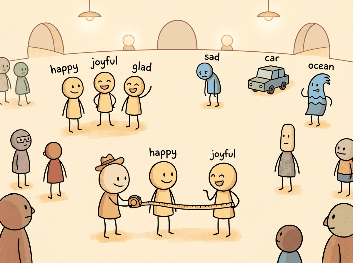
You shall know a word by the company it keeps.

Vec, Linguistically Social AI Agent

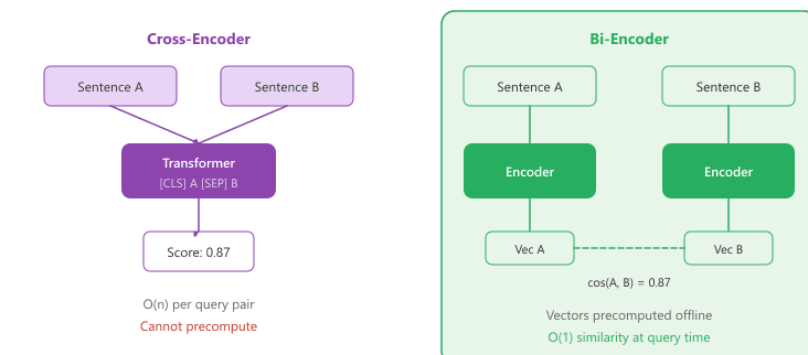
Contextual embeddings from transformer-based models like BERT resolved this ambiguity by producing different representations for the same word in different contexts. However, using BERT directly for sentence similarity proved problematic. Computing the similarity between two sentences required passing both through the model simultaneously (cross-encoding), making it computationally infeasible to search across millions of documents at query time.

The Bi-Encoder Architecture

The key innovation that made large-scale semantic search practical was the bi-encoder architecture, introduced by Sentence-BERT (SBERT) in 2019. Instead of feeding two sentences into one model jointly, the bi-encoder processes each sentence independently through the same transformer encoder, producing a fixed-size vector for each. These vectors can be precomputed and stored in an index, enabling similarity search with a simple dot product or cosine similarity operation at query time. contrasts these two architectures side by side.

Figure 31.1.2: Cross-encoder vs. bi-encoder architecture. The bi-encoder enables precomputation and fast similarity search.

Pooling Strategies

A transformer encoder produces one vector per input token. To obtain a single sentence-level vector, a pooling operation aggregates these token vectors. The three common strategies are:

• [CLS] token pooling: Use the output vector corresponding to the special classification token. This works well when the model has been specifically trained with a classification objective.
• Mean pooling: Average all token output vectors (excluding padding). This is the default for most modern sentence transformers and tends to produce the most robust representations, because it aggregates signal from every token position. Important information may be concentrated in different parts of the sentence, and averaging ensures none of it is lost. By contrast, the [CLS] token must compress the entire sentence into a single position during pretraining data, which may not happen effectively without explicit training for that purpose.
• Max pooling: Take the element-wise maximum across all token vectors. This can capture salient features but is less commonly used in practice.

# Encode three sentences with all-MiniLM-L6-v2 (a 384-dim mean-pooled model)
# and inspect pairwise cosine similarity for paraphrase vs. unrelated pairs.
from itertools import combinations
from sentence_transformers import SentenceTransformer

model = SentenceTransformer("sentence-transformers/all-MiniLM-L6-v2")
sentences = [
    "The cat sat on the mat.",
    "A feline rested on the rug.",      # paraphrase of sentence 0
    "Stock prices rose sharply today.",  # unrelated topic
]

# `normalize_embeddings=True` puts vectors on the unit sphere, so dot product == cosine.
embeddings = model.encode(sentences, normalize_embeddings=True)
print(f"Embedding shape: {embeddings.shape} (n_sentences, embed_dim)")

similarity = embeddings @ embeddings.T
for i, j in combinations(range(len(sentences)), 2):
    print(
        f"sim('{sentences[i][:30]}...', "
        f"'{sentences[j][:30]}...'): {similarity[i, j]:.4f}"
    )

pip install -U sentence-transformers
from sentence_transformers import SentenceTransformer

model = SentenceTransformer("BAAI/bge-m3", device="cuda")
embeddings = model.encode(
    ["The cat sat on the mat.", "A feline rested on the rug."],
    normalize_embeddings=True,
    batch_size=64,
)
# embeddings.shape == (2, 1024); cosine = embeddings @ embeddings.T

31.1.2 Training Embedding Models: Contrastive Learning

31.1.1 From Words to Sentences: The Embedding Evolution

In Section 1.3, we explored how words can be represented as dense vectors and how similarity metrics capture semantic relationships. This section builds on that foundation by showing how modern embedding models extend those ideas from individual words to entire sentences and paragraphs, enabling the large-scale semantic search that powers RAG systems.

The journey from word-level to sentence-level embeddings represents one of the most consequential progressions in NLP. Early approaches like Word2Vec and GloVe learned to map individual words into dense vectors where geometric relationships encoded semantic relationships. The classic example of king - man + woman ≈ queen demonstrated that these vector spaces captured meaningful analogies, but word embeddings suffered from a fundamental limitation: they assigned a single vector to each word regardless of context.

Modern embedding models are trained using contrastive learning, a framework where the model learns to pull similar (positive) pairs together and push dissimilar (negative) pairs apart in the embedding space. The quality of the training data, the choice of loss function, and the strategy for selecting hard negatives together determine the final embedding quality.

Loss Functions

Contrastive learning has several standard loss formulations. The two that dominate modern embedding training are Multiple Negatives Ranking Loss and Triplet Loss, with hard negative mining as a critical orthogonal technique that boosts both.

Multiple Negatives Ranking Loss (MNRL)

The most widely used loss function for embedding training is Multiple Negatives Ranking Loss (also called InfoNCE). Given a batch of N positive pairs (query, positive_passage), the loss treats the other N-1 passages in the batch as negatives for each query. This "in-batch negatives" approach is highly efficient because it provides N-1 negatives for free, without requiring explicit negative sampling.

Written out, for a query embedding $q$, its positive document $d^{+}$, and in-batch negatives $d^{-}_j$, the InfoNCE loss is

This is the cross-entropy of a softmax over similarities: retrieving the correct document is treated as a classification problem against the negatives. The temperature $\tau$ sharpens ($\tau \to 0$) or softens the distribution; a small $\tau$ forces the positive's similarity far above the negatives' but makes training more sensitive to hard negatives.

# Simplified InfoNCE / Multiple Negatives Ranking Loss
import torch
import torch.nn.functional as F
def multiple_negatives_ranking_loss(query_emb, passage_emb, temperature=0.05):
    """
    query_emb: (batch_size, embed_dim) - query embeddings
    passage_emb: (batch_size, embed_dim) - positive passage embeddings
    Each query_emb[i] pairs with passage_emb[i] (positive).
    All other passages in the batch serve as negatives.
    """
    # Compute similarity matrix: (batch_size, batch_size)
    similarity = torch.matmul(query_emb, passage_emb.T) / temperature
    # Labels: diagonal entries are the positives
    labels = torch.arange(similarity.size(0), device=similarity.device)
    # Cross-entropy loss treats this as N-way classification
    loss = F.cross_entropy(similarity, labels)
    return loss
# Example: batch of 4 query-passage pairs
batch_size, dim = 4, 384
queries = F.normalize(torch.randn(batch_size, dim), dim=-1)
passages = F.normalize(torch.randn(batch_size, dim), dim=-1)
loss = multiple_negatives_ranking_loss(queries, passages)
print(f"MNRL Loss: {loss.item():.4f}")

Triplet Loss and Other Objectives

Earlier approaches used triplet loss, which operates on (anchor, positive, negative) triples and enforces a margin between the positive and negative distances. While simpler conceptually, triplet loss is less sample-efficient than MNRL because it uses only one negative per anchor. Other loss variants include cosine similarity loss for regression-style training on continuous similarity scores, and distillation losses that transfer knowledge from a cross-encoder teacher to a bi-encoder student.

Hard Negative Mining

The choice of negative examples profoundly impacts embedding quality. Random negatives are typically too easy for the model to distinguish, providing little learning signal. Hard negatives are passages that are superficially similar to the query but are not actually relevant. They force the model to learn fine-grained distinctions.

# Hard negative mining: find passages that look relevant to a query but are not
# labeled as positive. Training on these tightens the model's decision boundary.
from sentence_transformers import SentenceTransformer
import numpy as np

def mine_hard_negatives(
    model: SentenceTransformer,
    queries: list[str],
    corpus: list[str],
    positives_map: dict[int, set[int]],
    top_k: int = 30,
    num_negatives: int = 5,
) -> dict[int, list[int]]:
    """For each query, return the top-k most similar non-positive corpus indices."""
    query_embs = model.encode(queries, normalize_embeddings=True)
    corpus_embs = model.encode(corpus, normalize_embeddings=True)
    hard_negatives = {}
    for q_idx, q_emb in enumerate(query_embs):
        # Cosine since embeddings are L2-normalized: dot product == cosine.
        sims = corpus_embs @ q_emb
        top_indices = np.argsort(sims)[::-1][:top_k]
        # Drop the labeled positives so what remains is "looks similar but is wrong".
        positives = positives_map.get(q_idx, set())
        neg_indices = [int(i) for i in top_indices if int(i) not in positives]
        hard_negatives[q_idx] = neg_indices[:num_negatives]
    return hard_negatives
# Example usage
model = SentenceTransformer("sentence-transformers/all-MiniLM-L6-v2")
queries = ["What causes diabetes?", "How does photosynthesis work?"]
corpus = [
    "Diabetes is caused by insulin resistance or insufficient insulin production.",
    "Type 2 diabetes risk factors include obesity and sedentary lifestyle.",
    "Photosynthesis converts sunlight into chemical energy in plants.",
    "The Calvin cycle fixes carbon dioxide into glucose molecules.",
    "Machine learning models require large datasets for training.",
    ]
positives_map = {0: {0, 1}, 1: {2, 3}}
negatives = mine_hard_negatives(model, queries, corpus, positives_map)
print("Hard negatives for each query:")
for q_idx, neg_ids in negatives.items():
    print(f" Query: '{queries[q_idx]}'")
    for nid in neg_ids:
        print(f" Negative: '{corpus[nid][:60]}...'")