Why have one head when you can have eight, each looking at the sentence from a slightly different existential angle?
Attn, Multi-Headed AI Agent
From seq2seq attention to the Transformer's attention. In Section 2.2, we used attention to let a decoder peek at encoder states. The Transformer (Vaswani et al., 2017) takes this much further. It introduces the query/key/value (Q/K/V) abstraction, scales the dot products by √$d_{k}$ for numerical stability, runs multiple attention "heads" in parallel, and applies attention not just between encoder and decoder but also within a single sequence (self-attention). These building blocks are the heart of GPT, BERT, and every modern LLM. By the end of this section, you will have implemented multi-head self-attention from scratch and understood every piece of the mechanism that makes Transformers work.
Q, K, V split one role into three: the query asks "what am I looking for?", the key answers "what do I contain?", the value says "what should I pass forward?" Multi-head attention runs this lookup eight times in parallel and concatenates, so each head can specialize in one type of relationship (syntax, coreference, position) without interfering with the others.
Prerequisites
This section assumes you understand the intuitive attention mechanism from Section 2.2 (alignment scores, weighted context vectors). Matrix multiplication and basic linear algebra (from Section 0.2) are needed for the Q/K/V formulation. The multi-head attention mechanism developed here is the core component of the Transformer architecture detailed in Section 3.1; for optimization-focused variants like grouped-query attention, see Section 3.3.

2.3.1 The Query, Key, Value Abstraction
The Q/K/V terminology was a deliberate database analogy from Vaswani et al. (2017), borrowed from the "associative memory" literature of the 1990s. The Transformer paper went through 6 working titles before "Attention Is All You Need", and the final title was reportedly an inside joke at a Google Brain meeting before it became the most-cited deep learning paper of the decade.
During training, the model at each position sees the true previous token from the ground-truth sequence (teacher forcing). At inference, that previous token is the model's own prediction, which may be wrong. If the model makes an error at step 5, step 6 now operates on input it never saw during training. Researchers call this exposure bias. It explains why models can produce fluent but hallucinated text: each token looks reasonable given local context, but small errors compound. Scheduled sampling (Bengio et al., 2015) and prefix-tuning approaches partially address this; no current training objective fully eliminates the gap. This is also why RLHF (which trains on model-generated sequences) tends to improve over SFT alone.
In Section 2.2, we described attention as a soft dictionary lookup: a query is compared against keys to produce weights, which are used to combine values. In Bahdanau and Luong attention, the keys and values were the same thing (encoder hidden states), and the query was the decoder state.
The Transformer formalizes and generalizes this. Given input vectors, it creates three separate representations through learned linear projections:
- Query (Q): What am I looking for? Obtained by projecting the input through $W^{Q}$.
- Key (K): What do I contain? Obtained by projecting the input through $W^{K}$.
- Value (V): What should I send back? Obtained by projecting the input through $W^{V}$.
These are separate projections of the same (or different) input vectors. This decoupling is crucial: the information used for matching (Q and K) can differ from the information that gets passed forward (V). A position might have a key that says "I am a verb in past tense" (used for matching) while its value encodes the actual semantic meaning of that verb (used for the output).
2.3.2 Scaled Dot-Product Attention
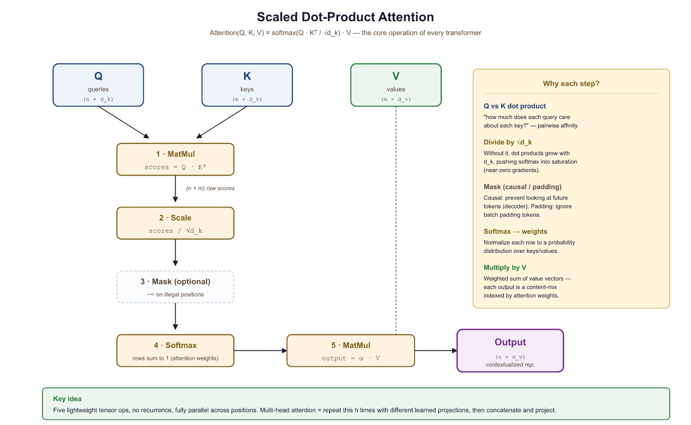
Given query matrix $Q$, key matrix $K$, and value matrix $V$, the Transformer computes:
Let us break this formula apart:
- QKT: Computes dot-product similarity between every query and every key simultaneously. If Q has shape $(n, d_{k})$ and K has shape $(m, d_{k})$, this produces an $(n, m)$ matrix of raw attention scores.
- Scaling by √$d_{k}$: Divides each score by the square root of the key dimension. Without this scaling, the dot products would grow in magnitude with $d_{k}$, pushing the softmax into saturated regions where its gradients are extremely small.
- Softmax: Converts each row into a probability distribution over key positions.
- Multiply by V: Uses the attention weights to take a weighted combination of value vectors.
Why Scale by √dk?
Without the √dk scaling, Transformers would barely train at all. The original "Attention Is All You Need" paper reports that unscaled dot-product attention produced significantly worse results. This single division operation is easy to overlook, but it is one of those small engineering decisions that makes the difference between a groundbreaking architecture and a failed experiment.
Consider two random vectors $q$ and $k$, each with entries drawn from a standard normal distribution. Their dot product
is a sum of $d_{k}$ independent products, each with mean 0 and variance 1. By the properties of sums of random variables, the dot product has mean 0 and variance $d_{k}$. As $d_{k}$ grows, the typical magnitude of the dot product increases as $\sqrt{d_k}$.
Large-magnitude inputs to softmax produce outputs very close to 0 or 1, with tiny gradients. Dividing by $\sqrt{d_k}$ restores the variance to approximately 1, keeping softmax in its sensitive, gradient-friendly regime.
# Show why scaling matters: as d_k grows, raw dot products explode
# and softmax saturates, concentrating all weight on one key.
import torch
import torch.nn.functional as F
torch.manual_seed(42)
# Demonstrate the scaling problem
for d_k in [8, 64, 512]:
    q = torch.randn(1, d_k)
    K = torch.randn(10, d_k)
    # Unscaled dot products
    scores_unscaled = q @ K.T
    # Scaled dot products
    scores_scaled = scores_unscaled / (d_k ** 0.5)
    probs_unscaled = F.softmax(scores_unscaled, dim=-1)
    probs_scaled = F.softmax(scores_scaled, dim=-1)
    print(f"d_k={d_k:3d} | unscaled std={scores_unscaled.std():.2f}, "
        f"max prob={probs_unscaled.max():.4f} | "
        f"scaled std={scores_scaled.std():.2f}, "
f"max prob={probs_scaled.max():.4f}")import torch
import torch.nn as nn
# Built-in MHA: same functionality, one line to create
mha = nn.MultiheadAttention(embed_dim=128, num_heads=4, batch_first=True)
x = torch.randn(2, 10, 128) # (batch, seq_len, d_model)
# Bidirectional (BERT-style): pass x as query, key, and value
out, weights = mha(x, x, x)
print(f"Output: {out.shape}") # torch.Size([2, 10, 128])
print(f"Weights: {weights.shape}") # torch.Size([2, 10, 10])
# Causal (GPT-style): generate a causal mask
mask = nn.Transformer.generate_square_subsequent_mask(10)
out_causal, _ = mha(x, x, x, attn_mask=mask)At $d_{k} = 512$, the unscaled softmax is completely saturated (max probability is essentially 1.0, meaning all attention goes to a single position). The scaled version maintains a healthy distribution. This is not just a cosmetic issue; saturated softmax means near-zero gradients, which makes training extremely difficult.
Scaling by $1/ \sqrt{d_k}$ is equivalent to using a softmax with temperature $T = \sqrt{d_k}$. Higher temperature produces softer (more uniform) distributions; lower temperature produces sharper (more peaked) ones. Some implementations allow an explicit temperature parameter for fine-grained control during inference, but during training the $\sqrt{d_k}$ scaling is standard.
The cleanest way to internalize scaled dot-product attention is to walk the formula through with tiny numbers. Consider a three-token sequence with $d_k = 2$ and these query, key, and value matrices (each row is one token):
Step 1: raw scores $QK^{T}$. Each entry $(i,j)$ is the dot product of query i with key j:
Step 2: scale by $\sqrt{d_k} = \sqrt{2} \approx 1.414$. Each entry is divided by that constant:
Step 3: row-wise softmax. Each row becomes a probability distribution. For row 1 the unnormalized exponentials are $(e^{0.707}, e^{0}, e^{0.707}) \approx (2.028, 1.000, 2.028)$, which sum to $5.056$ and normalize to $(0.401, 0.198, 0.401)$. Repeating for the other two rows:
Step 4: weighted sum of values. Each output row is the attention-weighted combination of the rows of $V$. For row 1: $0.401 \cdot (10,0) + 0.198 \cdot (0,10) + 0.401 \cdot (5,5)$ $= (4.01, 0) + (0, 1.98) + (2.01, 2.01) = (6.02, 3.99)$. Repeating for all rows:
Three things to notice. First, the diagonal of the score matrix is highest, because each token's query best matches its own key; this is why a token always pays the most attention to itself in self-attention. Second, the third token, whose query vector $(1,1)$ aligns with both keys, ends up with an output that is a near-uniform mix of all three values. Third, removing the $\sqrt{d_k}$ divisor would push the row-3 softmax toward $(0.21, 0.21, 0.58)$, sharper but with smaller gradients; with much larger $d_k$ the unscaled softmax would collapse to a one-hot row, which is the saturation pathology illustrated numerically above.
Implementation from Scratch
This implementation computes scaled dot-product attention step by step, including the optional causal mask.
# Scaled dot-product attention from scratch: Q @ K^T / sqrt(d_k),
# optional mask to block future tokens, softmax, then V weighting.
import torch
import torch.nn.functional as F
import math
def scaled_dot_product_attention(Q, K, V, mask=None):
    """
    Q: (batch, n_queries, d_k)
    K: (batch, n_keys, d_k)
    V: (batch, n_keys, d_v)
    mask: (batch, n_queries, n_keys) or broadcastable, True = mask out
    Returns: output (batch, n_queries, d_v), weights (batch, n_queries, n_keys)
    """
    d_k = Q.size(-1)
    # Step 1: Compute raw attention scores
    scores = torch.bmm(Q, K.transpose(-2, -1)) # (batch, n_q, n_k)
    # Step 2: Scale
    scores = scores / math.sqrt(d_k)
    # Step 3: Apply mask (if provided)
    if mask is not None:
        scores = scores.masked_fill(mask, float('-inf'))
        # Step 4: Softmax to get attention weights
        weights = F.softmax(scores, dim=-1) # (batch, n_q, n_k)
        # Step 5: Weighted sum of values
        output = torch.bmm(weights, V) # (batch, n_q, d_v)
        return output, weights
        # Test: 4 queries attending to 6 key-value pairs
        batch, n_q, n_k, d_k, d_v = 2, 4, 6, 32, 64
        Q = torch.randn(batch, n_q, d_k)
        K = torch.randn(batch, n_k, d_k)
        V = torch.randn(batch, n_k, d_v)
        out, wts = scaled_dot_product_attention(Q, K, V)
        print(f"Output shape: {out.shape}") # (2, 4, 64)
        print(f"Weights shape: {wts.shape}") # (2, 4, 6)
        print(f"Weights row 0 sums to: {wts[0, 0].sum():.4f}")
print(f"Weights[0,0]: {wts[0,0].detach().numpy().round(3)}")The $\sqrt{d_k}$ divisor is the most consequential typographical decision in deep learning. Forget it, and a 512-dim attention layer produces dot products in the hundreds, softmax slams every weight to either 0 or 1, gradients vanish, and your model learns nothing. Include it, and dot products stay near unit variance, softmax stays in its informative middle zone, and the architecture trains. The entire LLM revolution turns on one square root. If a typo had dropped that radical sign in 2017, we would still be writing LSTMs.
2.3.3 Self-Attention vs. Cross-Attention
The Q/K/V framework enables two fundamental modes of attention:
Self-Attention
In self-attention, the queries, keys, and values all come from the same sequence. Each position in the sequence attends to every other position (including itself). This allows each token to gather information from the entire input, building context-aware representations in a single operation.
Self-attention is what makes Transformers fundamentally different from RNNs. An RNN can only see past context (or future context, if bidirectional); self-attention sees all positions simultaneously. For a sentence like "The animal didn't cross the street because it was too tired," self-attention allows the model to connect "it" directly to "animal" regardless of distance.
Cross-Attention
In cross-attention, the queries come from one sequence (typically the decoder) while the keys and values come from a different sequence (typically the encoder). This is exactly the encoder-decoder attention from Section 2.2, reformulated in the Q/K/V framework. Cross-attention is what allows a Transformer decoder to "look at" the encoder output.
| Property | Self-Attention | Cross-Attention |
|---|---|---|
| Q source | Same sequence (X) | Decoder states |
| K, V source | Same sequence (X) | Encoder outputs |
| Typical use | Build contextual representations | Combine encoder/decoder information |
| Score matrix shape | (n, n), square | ($n_{dec}$, $n_{enc}$), rectangular |
| Examples | BERT, GPT encoder/decoder blocks | Machine translation, T5 decoder |
2.3.4 Causal Masking for Autoregressive Models
In autoregressive language models (like GPT), each token should only attend to tokens
that appear before it in the sequence (and itself). It must not "peek" at future
tokens that have not been generated yet. This causal constraint is what makes left-to-right text generation (Chapter 4) possible. This constraint is enforced with a
causal mask: an upper-triangular matrix of True values
that sets future positions to $- \infty$ before the softmax.
After masking, the scores for future positions become $- \infty$, which softmax maps to exactly 0. Each position can only attend to itself and earlier positions.
# Causal (autoregressive) masking: build an upper-triangular boolean mask
# and pass it to scaled_dot_product_attention to block future positions.
import torch
# Create a causal mask for sequence length 5
seq_len = 5
causal_mask = torch.triu(torch.ones(seq_len, seq_len, dtype=torch.bool), diagonal=1)
print("Causal mask (True = blocked):")
print(causal_mask.int())
# Apply to attention scores
scores = torch.randn(1, seq_len, seq_len)
# Mask future positions with -inf so softmax ignores them
scores_masked = scores.masked_fill(causal_mask.unsqueeze(0), float('-inf'))
# Convert scores to attention weights (probabilities summing to 1)
weights = torch.softmax(scores_masked, dim=-1)
print("\nAttention weights (causal):")
print(weights[0].detach().numpy().round(3))Notice the triangular structure: position 0 can only attend to itself (weight 1.0), position 1 can attend to positions 0 and 1, and so on. The upper triangle is exactly zero, guaranteeing no information leakage from the future.
Causal masking is what distinguishes GPT-style (decoder-only) models from BERT-style (encoder-only) models. BERT uses bidirectional self-attention (no mask), so every position can attend to every other position. GPT uses causal self-attention (with mask), so each position can only see the past. This difference determines what tasks each architecture is suited for: BERT excels at understanding (classification, NER), while GPT excels at generation (text completion, dialogue).
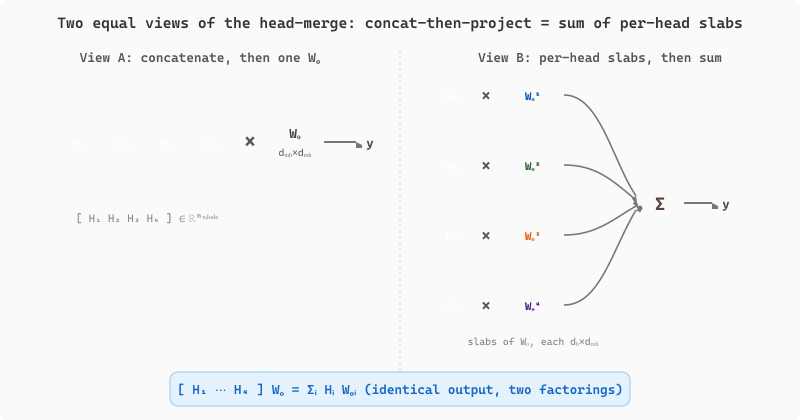
A common point of confusion is whether multi-head attention is "really" $h$ independent attentions glued together, or whether the trailing $W_O$ projection does meaningful work. The math says: it is both, and the $W_O$ is doing more than reshape. Let each head $i \in \{1, \ldots, h\}$ produce output $H_i \in \mathbb{R}^{n \times d_h}$ where $d_h = d_{\text{model}} / h$. The standard multi-head formula is
where $W_O \in \mathbb{R}^{d_{\text{model}} \times d_{\text{model}}}$ and the second equality block-decomposes $W_O$ into $h$ vertical slabs $W_O^{(i)} \in \mathbb{R}^{d_h \times d_{\text{model}}}$, one per head. The right-hand side makes the architecture's intent explicit: each head $i$ writes its output $H_i$ into the residual stream through its own projection $W_O^{(i)}$. The heads' subspaces are disjoint in the concatenation but they are recombined into the residual through $W_O$, which is learned end-to-end. Because $W_O$ has $d_{\text{model}}^2$ parameters (not $h$ separate $d_h \times d_h$ matrices), it can mix information across heads at the output, not just within a head. If you replaced $W_O$ with the identity, the heads would have to write into disjoint slices of the residual stream and could never interact at this layer; with $W_O$ trained, the heads can be thought of as $h$ proposed updates that the linear combiner $W_O$ blends into a single coherent write.
This block-decomposition view also explains why sharing $W_Q, W_K, W_V$ across heads (Exercise 2.3.3) defeats the purpose. If every head computes the same attention pattern, then $H_1 = H_2 = \cdots = H_h$, and the sum $\sum_i H_i W_O^{(i)} = H_1 \cdot (\sum_i W_O^{(i)})$ collapses to a single rank-$d_h$ update with $\sum_i W_O^{(i)}$ as its projection. The model has $h\times$ the per-head compute of single-head attention but exactly the representational capacity of one wider head; training would converge to the same loss as a model with $h = 1$ and $d_h \to d_{\text{model}}$. The win from multi-head only materializes when the heads compute different attention patterns, which is why $W_Q, W_K, W_V$ are typically realized as one large $d_{\text{model}} \times d_{\text{model}}$ projection that is then sliced into per-head matrices: the slicing forces the heads to live in disjoint subspaces, and training shapes each subspace toward a different relationship type (syntactic, semantic, positional). The linearity proof in this paragraph also shows why post-softmax operations such as RoPE (Section 3.5) commute correctly with the head structure: the rotation acts within each head's $d_h$-dimensional Q/K subspace and $W_O$ recombines the rotated outputs, so the head-merge step does not reintroduce position dependence after the fact. Reference: Vaswani et al., "Attention Is All You Need," arXiv:1706.03762 (2017), Sec. 3.2.2.
Figure 2.3.3 shows the two equivalent views of the head-merge step side by side: concatenating the per-head outputs and applying one big $W_O$ (left) is exactly equal to projecting each head through its own horizontal slab $W_O^{(i)}$ and summing (right).
Reproduce the scaling demonstration: draw q and K from a standard normal with d_k in {8, 64, 512, 4096}, compute both unscaled and scaled softmax over a 10-key row, and report (a) the empirical std of the dot products and (b) the max softmax probability. Verify that scaled std stays near 1.0 and max prob stays under 0.30 for all d_k.
Answer Sketch
Expected: unscaled std grows as sqrt(d_k) (about 2.8, 8, 22.6, 64), and max softmax probability saturates near 1.0 for d_k >= 64. After dividing by sqrt(d_k), std remains around 1.0 and max prob stays in the 0.2 to 0.3 range. This is the gradient-friendly regime that lets the network actually learn.
Given a sequence of length 6, construct the causal attention mask as a (6, 6) tensor where entry (i, j) = 0 for j <= i and -inf for j > i. Apply softmax over the masked scores from a random (6, 6) score matrix and assert that each row's probability sums to 1 and that all upper-triangular entries are exactly zero.
Answer Sketch
Use torch.triu(torch.ones(6, 6), diagonal=1).bool() and scores.masked_fill_(mask, float('-inf')). After softmax, row sums are 1.0 (up to float precision); entries above the diagonal are 0.0 because exp(-inf) = 0. If the test fails, the most likely cause is masking with a large negative number like -1e9 in mixed precision, where exp(-1e9) = 0 only in float32, not in float16.
You implement multi-head attention but, as a "simplification", reuse the same W_Q, W_K, W_V across all 8 heads (instead of one set per head). Predict what happens during training and explain why this defeats the purpose of multi-head attention.
Answer Sketch
All heads compute identical attention patterns, so concatenating them is redundant. The model has 8x the per-token compute of single-head attention but no extra representational capacity. In practice you would see no improvement over a wider single-head attention, and training would converge to the same loss as a model with num_heads=1 and 8x larger d_head. The whole point of multi-head is that each head learns a different subspace.
What's Next?
In the next part of this section, Section 2.4: Multi-Head Attention, Complexity & Lab, the query-key-value abstraction, scaled dot-product attention, self vs cross attention, and causal masking for autoregressive models.