I built a Transformer from scratch and it predicted "the the the the." Honestly, some meetings feel the same way.
Norm, Repetitively Decoded AI Agent
Reading about attention heads and layer normalization is one thing; implementing them is another. This hands-on lab translates the architecture from Section 3.1 into working PyTorch code, building a character-level language model step by step. By the end, you will have internalized how data flows through embeddings, multi-head attention, and feed-forward layers. This concrete understanding pays dividends when you fine-tune models in Chapter 16 or debug inference issues in production.
Prerequisites
This coding lab requires a solid understanding of the Transformer architecture from Section 3.1 and layer normalization from Section 2.3. You will write PyTorch code, so the PyTorch tutorial in Section 0.3 (tensors, autograd, training loops) is essential preparation.
This section is a coding lab. By the end you will have a working character-level language model built on a decoder-only Transformer. Every line of code is explained. We encourage you to type the code yourself rather than copy-pasting; the act of typing builds muscle memory for these patterns.

3.3.1 What We Are Building
The character-level mini-Transformer recipe we are about to build is essentially Andrej Karpathy's nanoGPT, which trains Shakespeare in under 3 minutes on a single GPU. nanoGPT is under 300 lines and has been re-implemented in Rust, C, Mojo, and at least one esoteric language called Brainfuck (for sport). The Mojo version was used in 2024 to win an internal Modular hackathon.
The QKV mechanism is a differentiable key-value store. Queries retrieve values by weighted similarity across all keys, exactly like a fuzzy database lookup. Unlike SQL, attention has no "null result": when no key closely matches the query, it still returns a weighted average of all values, weighted by imperfect similarity. This is the root cause of attention-based confabulation: the model retrieves a plausible but incorrect "nearest match" rather than reporting uncertainty. The KV cache (Chapter 10) is, from this perspective, simply a precomputed cache of database rows, subject to the same latency-versus-memory tradeoffs as any database cache.
We will implement a decoder-only Transformer (the GPT architecture) that performs character-level language modeling. Given a sequence of characters, the model predicts the next character at every position. We choose character-level modeling because it eliminates the need for a tokenizer (Chapter 1), letting us focus entirely on the architecture.
Our model will have these hyperparameters:
| Hyperparameter | Value | Notes |
|---|---|---|
| d_model | 128 | Embedding and residual stream dimension |
| n_heads | 4 | Number of attention heads (d_k = 32) |
| n_layers | 4 | Number of Transformer blocks |
| d_ff | 512 | Feed-forward inner dimension (4 × d_model) |
| block_size | 128 | Maximum context length |
| vocab_size | ~65 | Unique characters in the dataset |
| dropout | 0.1 | Dropout rate |
This is a small model (~1.6M parameters) that trains in a few minutes on a single GPU (or even on CPU for a few epochs). The architecture is identical to GPT; only the scale differs.
Typing each line yourself forces you to read and understand every operation. You will notice patterns (the repeated LayerNorm, the residual connections, the projection matrices) that become invisible when you copy-paste. These patterns are the same ones you will encounter in every production Transformer codebase, from Hugging Face to vLLM.
3.3.2 The Complete Implementation
Below is the full model in a single file. We break it into logical pieces and explain each one. The complete code (all pieces assembled) is approximately 300 lines including comments.
3.3.2.1 Imports and Configuration
We begin by importing PyTorch and defining a configuration dataclass that holds all model hyperparameters.
"""
mini_transformer.py
A minimal decoder-only Transformer for character-level language modeling.
~300 lines of annotated PyTorch.
"""
import math
import torch
import torch.nn as nn
import torch.nn.functional as F
from dataclasses import dataclass, asdict

@dataclass
class TransformerConfig:
    """All hyperparameters in one place."""
    vocab_size: int = 65          # number of unique characters
    block_size: int = 128         # maximum context length
    n_layers: int = 4             # number of Transformer blocks
    n_heads: int = 4              # number of attention heads
    d_model: int = 128            # embedding / residual stream dimension
    d_ff: int = 512               # feed-forward inner dimension
    dropout: float = 0.1           # dropout probability
    bias: bool = False             # use bias in Linear layers?

def describe(cfg: TransformerConfig) -> None:
    """Pretty-print the config so you see every knob in one place."""
    for k, v in asdict(cfg).items():
        print(f"  {k:12s} = {v}")

cfg = TransformerConfig()
describe(cfg)
We use a dataclass so that every hyperparameter is explicit, documented, and easy to
modify. Setting bias=False follows the LLaMA convention and marginally reduces
parameter count.
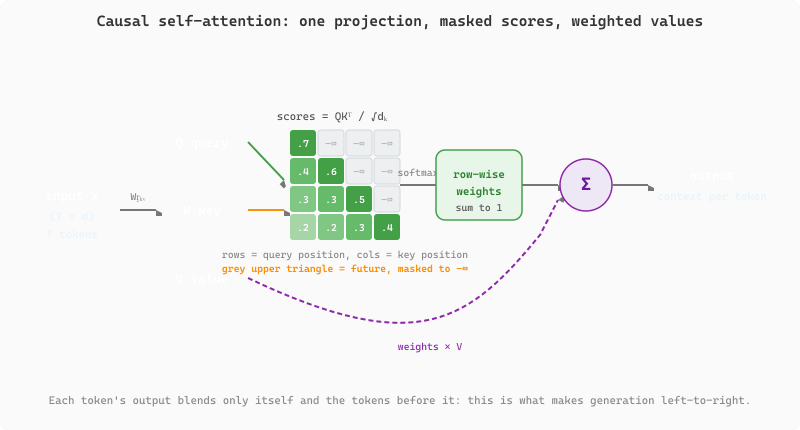
3.3.2.2 Causal Self-Attention
This module implements multi-head causal self-attention with a triangular mask that prevents positions from attending to future tokens. Figure 3.3.3 traces the data flow that the code below implements: one projection splits each token into a query, key, and value, the scaled dot-product of queries and keys forms an attention score grid, and a lower-triangular mask zeroes out every future position before softmax so each token can only mix information from itself and earlier tokens.
torch.tril mask registered as a buffer in the code below.import torch.nn.functional as F
from torch import nn
import torch
# Causal self-attention with a triangular mask: each token can only
# attend to itself and earlier positions, enforcing left-to-right generation.
class CausalSelfAttention(nn.Module):
"""Multi-head causal (masked) self-attention."""
def __init__(self, config: TransformerConfig):
super().__init__()
assert config.d_model % config.n_heads == 0
# Key, Query, Value projections combined into one matrix
self.qkv_proj = nn.Linear(config.d_model, 3 * config.d_model, bias=config.bias)
# Output projection
self.out_proj = nn.Linear(config.d_model, config.d_model, bias=config.bias)
self.attn_dropout = nn.Dropout(config.dropout)
self.resid_dropout = nn.Dropout(config.dropout)
self.n_heads = config.n_heads
self.d_model = config.d_model
self.d_k = config.d_model // config.n_heads
# Causal mask: lower-triangular boolean matrix
# Register as buffer so it moves to GPU with the model
mask = torch.tril(torch.ones(config.block_size, config.block_size))
self.register_buffer("mask", mask.view(1, 1, config.block_size, config.block_size))
def forward(self, x):
B, T, C = x.shape # batch, sequence length, d_model
# Compute Q, K, V in one matrix multiply, then split
qkv = self.qkv_proj(x)
q, k, v = qkv.split(self.d_model, dim=2)
# Reshape for multi-head: (B, T, C) -> (B, n_heads, T, d_k)
q = q.view(B, T, self.n_heads, self.d_k).transpose(1, 2)
k = k.view(B, T, self.n_heads, self.d_k).transpose(1, 2)
v = v.view(B, T, self.n_heads, self.d_k).transpose(1, 2)
# Scaled dot-product attention
# (B, n_heads, T, d_k) @ (B, n_heads, d_k, T) -> (B, n_heads, T, T)
scores = (q @ k.transpose(-2, -1)) * (self.d_k ** -0.5)
# Apply causal mask: positions beyond current token get -inf
scores = scores.masked_fill(self.mask[:, :, :T, :T] == 0, float('-inf'))
attn_weights = F.softmax(scores, dim=-1)
attn_weights = self.attn_dropout(attn_weights)
# Weighted sum of values
# (B, n_heads, T, T) @ (B, n_heads, T, d_k) -> (B, n_heads, T, d_k)
out = attn_weights @ v
# Concatenate heads: (B, n_heads, T, d_k) -> (B, T, C)
out = out.transpose(1, 2).contiguous().view(B, T, C)
# Final linear projection + dropout
return self.resid_dropout(self.out_proj(out))
CausalSelfAttention(TransformerConfig(...)) and call on a tensor of shape (B, T, d_model) to produce a tensor of the same shape; the causal mask zeroes out attention to future positions.)
Notice the line scores = (q @ k.transpose(-2, -1)) * (self.d_k ** -0.5). That
** -0.5 term (equivalent to dividing by √dk) is not cosmetic; it
prevents softmax from collapsing into a near-one-hot distribution.
Here is why. If the entries of Q and K are drawn roughly from a standard normal distribution (mean 0, variance 1), then each element of the dot product Q·K is the sum of dk products of independent unit-normal variables. By the properties of variance, the dot product has variance dk. For our config with dk = 32, this means raw scores have a standard deviation around 5 to 6. For a larger model with dk = 128, the standard deviation grows to about 11.
Feed values that large into softmax and the result becomes near-one-hot: almost all the attention weight concentrates on a single position, and the gradients of all other positions effectively vanish. The model stops learning. Dividing by √dk rescales the scores back to unit variance, keeping the softmax in a numerically healthy region where it produces diffuse distributions and carries gradients to all attended positions.
Concrete example: with dk = 128 and no scaling, a single score might be 14 while others cluster around 0. softmax(14, 0, 0, …) ≈ (0.9999, 0.00003, …). After dividing by √128 ≈ 11.3, the same score becomes ~1.2, and softmax produces a much more spread-out distribution where all positions can receive meaningful gradient signal. Section 3.5 explores how RoPE and other positional encodings interact with this scaling.
Our config uses n_heads=4, splitting dmodel=128 into four 32-dimensional
subspaces. Why not just do one big attention over all 128 dimensions?
Each head learns to attend to a different kind of relationship simultaneously. In a trained language model, different heads specialize in distinct patterns. Some heads focus on syntactic relationships: the subject attending to its verb, or a pronoun attending to its antecedent. Other heads capture positional patterns: attending to the immediately preceding token or to the first token in the sequence (a common "global anchor" behavior). Still others detect semantic similarity: tokens that occur in similar contexts across the corpus attracting one another.
If you used a single attention head over the full dmodel-dimensional space, the
attention weight at each position is a single scalar. Multiple heads produce
n_heads independent attention distributions over the sequence; the concatenation
of their weighted value outputs gives the model the ability to simultaneously retrieve
information along all these different relational axes. The output projection WO
then integrates these parallel "views" into a single updated representation.
Clark et al. (2019) visualized BERT's attention heads and found that individual heads develop
highly interpretable functions: one head predominantly attends to the
[SEP] separator token (global context anchor), another tracks direct objects of
verbs, and another follows coreference chains. These specializations emerge from training
alone; they are not explicitly programmed. See
Section 3.5 for more on attention head behavior.
Many readers assume each head sees the full dmodel-dimensional representation and that "8 heads" means "8 times the work of 1 head." Actually, each head operates on a dmodel/n_heads slice (32 dims for 4 heads on a 128-dim model), so the total FLOPs are the same as a single full-width attention. What multi-head buys you is the freedom to learn n_heads different similarity functions in parallel from disjoint subspaces; you are not paying more compute, you are spending the same compute more diversely.
We compute Q, K, and V with a single linear layer (qkv_proj) of size
d_model → 3 * d_model and then split the output into three equal parts.
This is mathematically identical to three separate linear layers but is more efficient because
it performs one large matrix multiply instead of three smaller ones. The GPU utilizes its
parallelism more effectively with larger matrices.
3.3.2.3 Feed-Forward Network
The position-wise feed-forward network applies two linear transformations with a nonlinearity in between.
import torch.nn.functional as F
from torch import nn
# Position-wise FFN: expand to 4*d_model with ReLU, then project back.
# Applied independently at every token position in the sequence.
class FeedForward(nn.Module):
    """Position-wise feed-forward network with ReLU activation."""
    def __init__(self, config: TransformerConfig):
        super().__init__()
        self.fc1 = nn.Linear(config.d_model, config.d_ff, bias=config.bias)
        self.fc2 = nn.Linear(config.d_ff, config.d_model, bias=config.bias)
        self.dropout = nn.Dropout(config.dropout)
        # Forward pass: define computation graph
    def forward(self, x):
        x = F.relu(self.fc1(x))
        x = self.dropout(x)
        x = self.fc2(x)
        x = self.dropout(x)
        return x
This is the simplest version. For a more advanced variant, you can swap in SwiGLU.
import torch.nn.functional as F
from torch import nn
# SwiGLU FFN variant (LLaMA, PaLM): replace ReLU with a gated SiLU
# activation, using 2/3 of the hidden dimension for the gate projection.
class SwiGLUFeedForward(nn.Module):
    """SwiGLU feed-forward (used in LLaMA, PaLM)."""
    def __init__(self, config: TransformerConfig):
        super().__init__()
        # SwiGLU uses 3 weight matrices instead of 2
        # To keep param count comparable, the hidden dim is often 2/3 of d_ff
        hidden = int(2 * config.d_ff / 3)
        self.w1 = nn.Linear(config.d_model, hidden, bias=config.bias)
        self.w2 = nn.Linear(hidden, config.d_model, bias=config.bias)
        self.w3 = nn.Linear(config.d_model, hidden, bias=config.bias) # gate
        self.dropout = nn.Dropout(config.dropout)
    def forward(self, x):
        # SiLU(x * W1) * (x * W3) then project back
        return self.dropout(self.w2(F.silu(self.w1(x)) * self.w3(x)))
3.3.2.4 Transformer Block
Each block combines causal self-attention and a feed-forward network with residual connections and layer normalization.
from torch import nn
# Single transformer block: Pre-LN ordering with residual connections.
# Input flows through norm, attention, add residual, norm, FFN, add residual.
class TransformerBlock(nn.Module):
    """A single Transformer block with Pre-LN ordering."""
    def __init__(self, config: TransformerConfig):
        super().__init__()
        self.ln1 = nn.LayerNorm(config.d_model)
        self.attn = CausalSelfAttention(config)
        self.ln2 = nn.LayerNorm(config.d_model)
        self.ffn = FeedForward(config)
        # Forward pass: define computation graph
    def forward(self, x):
        # Pre-LN: normalize before each sub-layer
        x = x + self.attn(self.ln1(x)) # residual + attention
        x = x + self.ffn(self.ln2(x)) # residual + FFN
        return x
This is remarkably simple. Two lines of actual computation, each following the pattern:
x = x + SubLayer(LayerNorm(x)). The softmax is the x + at the
beginning; the Pre-LN ordering means we normalize the input to each sub-layer, not the output.
The original "Attention Is All You Need" paper (Vaswani et al., 2017) placed LayerNorm
after the residual add: LayerNorm(x + SubLayer(x)). This is called
Post-LN. Our implementation uses Pre-LN: x + SubLayer(LayerNorm(x)).
That subtle reordering has a large practical effect.
With Post-LN, the gradients flowing back through the network must pass through the LayerNorm before reaching earlier layers. This creates large gradient variance that makes training unstable at large scale, requiring careful learning-rate warmup schedules. Pre-LN sends the raw residual gradient directly back to all earlier layers without passing through the norm, resulting in much more stable gradient flow. Virtually every modern LLM (GPT-2 onward, LLaMA, Mistral, Gemma) uses Pre-LN as a result.
There is also a simplified variant called RMSNorm (Zhang & Sennrich, 2019) that removes the mean-centering step of standard LayerNorm, keeping only the root-mean-square scaling. This reduces computation slightly with no measurable quality loss and is used in LLaMA, Mistral, and Qwen. For a full comparison of Post-LN, Pre-LN, and RMSNorm, including an architecture diagram, see Section 3.5a: Pre-Norm vs. Post-Norm.
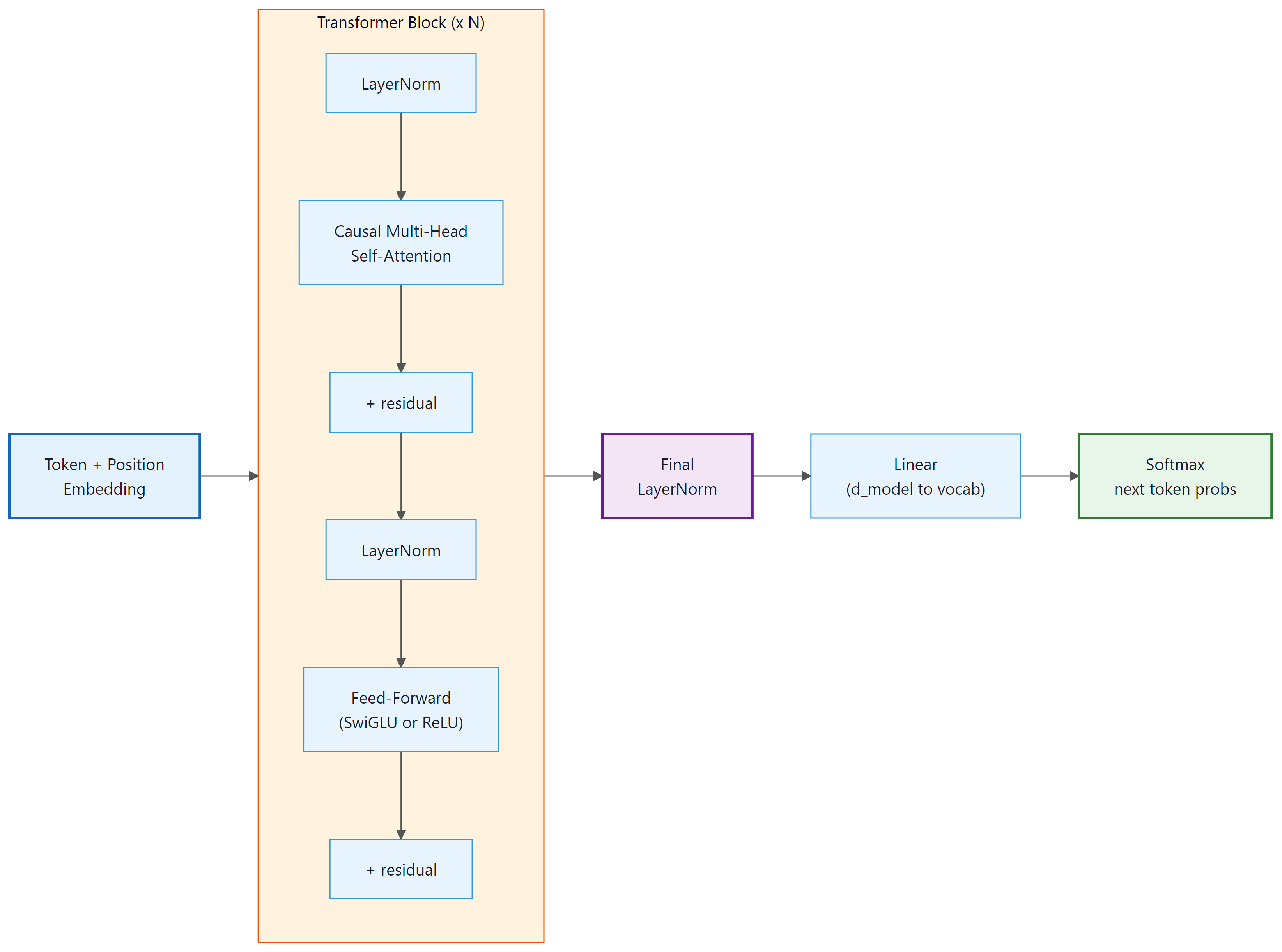
3.3.2.5 The Complete Model
The full model stacks an embedding layer, multiple Transformer blocks, and a final linear head for next-token prediction.
import torch.nn.functional as F
import math
from torch import nn
import torch
# Full decoder-only transformer: stack N blocks, add token + position
# embeddings, project to vocabulary logits, and implement autoregressive generate().
class MiniTransformer(nn.Module):
    """Decoder-only Transformer for character-level language modeling."""
    def __init__(self, config: TransformerConfig):
        super().__init__()
        self.config = config
        # Token and position embeddings
        self.token_emb = nn.Embedding(config.vocab_size, config.d_model)
        self.pos_emb = nn.Embedding(config.block_size, config.d_model)
        self.drop = nn.Dropout(config.dropout)
        # Stack of Transformer blocks
        self.blocks = nn.ModuleList([
            TransformerBlock(config) for _ in range(config.n_layers)
            ])
        # Final layer norm (needed with Pre-LN)
        self.ln_final = nn.LayerNorm(config.d_model)
        # Output head: project from d_model to vocab_size
        self.lm_head = nn.Linear(config.d_model, config.vocab_size, bias=False)
        # Weight tying: share embedding and output weights
        self.token_emb.weight = self.lm_head.weight
        # Initialize weights
        self.apply(self._init_weights)
        # Scale residual projections
        for block in self.blocks:
            nn.init.normal_(
                block.attn.out_proj.weight,
                mean=0.0,
                std=0.02 / math.sqrt(2 * config.n_layers)
                )
            nn.init.normal_(
                block.ffn.fc2.weight,
                mean=0.0,
                std=0.02 / math.sqrt(2 * config.n_layers)
                )
    def _init_weights(self, module):
        if isinstance(module, nn.Linear):
            nn.init.normal_(module.weight, mean=0.0, std=0.02)
            if module.bias is not None:
                nn.init.zeros_(module.bias)
            elif isinstance(module, nn.Embedding):
                nn.init.normal_(module.weight, mean=0.0, std=0.02)
            elif isinstance(module, nn.LayerNorm):
                nn.init.ones_(module.weight)
                nn.init.zeros_(module.bias)
    def forward(self, idx, targets=None):
        """
    Args:
    idx: (B, T) tensor of token indices
    targets: (B, T) tensor of target token indices (optional)
    Returns:
    logits: (B, T, vocab_size)
    loss: scalar cross-entropy loss (only if targets provided)
    """
        B, T = idx.shape
        assert T <= self.config.block_size, \
        f"Sequence length {T} exceeds block_size {self.config.block_size}"
        # Token embeddings + positional embeddings
        positions = torch.arange(0, T, device=idx.device) # (T,)
        x = self.token_emb(idx) + self.pos_emb(positions) # (B, T, d_model)
        x = self.drop(x)
        # Pass through all Transformer blocks
        for block in self.blocks:
            x = block(x)
            # Final normalization
            x = self.ln_final(x)
            # Project to vocabulary
            logits = self.lm_head(x) # (B, T, vocab_size)
            # Compute loss if targets are provided
            loss = None
            if targets is not None:
                loss = F.cross_entropy(
                    logits.view(-1, logits.size(-1)),
                    targets.view(-1)
                    )
                return logits, loss
    @torch.no_grad()
    def generate(self, idx, max_new_tokens, temperature=1.0, top_k=None):
        """
    Auto-regressive generation.
    Args:
    idx: (B, T) conditioning sequence
    max_new_tokens: number of tokens to generate
    temperature: softmax temperature (lower = more deterministic)
    top_k: if set, only sample from top-k most likely tokens
    """
        for _ in range(max_new_tokens):
            # Crop context to block_size if needed
            idx_cond = idx[:, -self.config.block_size:]
            # Forward pass
            logits, _ = self(idx_cond)
            # Take logits at the last position and apply temperature
            logits = logits[:, -1, :] / temperature
            # Optional top-k filtering
            if top_k is not None:
                v, _ = torch.topk(logits, min(top_k, logits.size(-1)))
                logits[logits < v[:, [-1]]] = float('-inf')
                # Sample from the distribution
                probs = F.softmax(logits, dim=-1)
                next_token = torch.multinomial(probs, num_samples=1)
                # Append to sequence
                idx = torch.cat([idx, next_token], dim=1)
                return idx
# Weight initialization + autoregressive text generation for our mini-Transformer.
# Add these methods to the MiniTransformer class from earlier.
import torch
import torch.nn as nn

def _init_weights(self, module: nn.Module) -> None:
    """Recommended init for transformers: small Gaussian for Linear/Embedding,
    zeros for biases. Call self.apply(self._init_weights) from __init__."""
    if isinstance(module, nn.Linear):
        nn.init.normal_(module.weight, mean=0.0, std=0.02)
        if module.bias is not None:
            nn.init.zeros_(module.bias)
    elif isinstance(module, nn.Embedding):
        nn.init.normal_(module.weight, mean=0.0, std=0.02)
    elif isinstance(module, nn.LayerNorm):
        nn.init.ones_(module.weight)
        nn.init.zeros_(module.bias)

@torch.no_grad()
def generate(self, idx: torch.Tensor, max_new_tokens: int,
             temperature: float = 1.0, top_k: int | None = None) -> torch.Tensor:
    """Autoregressively extend the (B, T) integer tensor `idx`.
    Returns a (B, T + max_new_tokens) tensor."""
    self.eval()
    for _ in range(max_new_tokens):
        # Crop to the last block_size tokens (context window limit)
        idx_cond = idx[:, -self.block_size:]
        logits = self(idx_cond)                # (B, T, vocab)
        logits = logits[:, -1, :] / temperature  # last position only
        if top_k is not None:
            v, _ = torch.topk(logits, top_k)
            logits[logits < v[:, [-1]]] = float("-inf")
        probs = torch.softmax(logits, dim=-1)
        next_id = torch.multinomial(probs, num_samples=1)   # (B, 1)
        idx = torch.cat([idx, next_id], dim=1)
return idx_init_weights) and autoregressive text generation (generate) for the mini-Transformer. Apply _init_weights via self.apply(self._init_weights) from __init__; call generate with a context tensor to produce new tokens with temperature/top-k sampling.The implementation above builds a complete decoder-only Transformer from scratch for pedagogical clarity. In production, use Hugging Face Transformers (install: pip install transformers), which provides pretrained models and a standardized API (see Code Fragment 3.3.8 below).
# Production equivalent: load a pre-trained causal LM
from transformers import AutoModelForCausalLM, AutoTokenizer
model = AutoModelForCausalLM.from_pretrained("gpt2")
tokenizer = AutoTokenizer.from_pretrained("gpt2")
inputs = tokenizer("The future of AI", return_tensors="pt")
output = model.generate(**inputs, max_new_tokens=50, temperature=0.8)
print(tokenizer.decode(output[0]))
The generate method above uses temperature and top-k sampling, two of the core decoding strategies explored in depth in Chapter 4: Decoding and Text Generation. The line self.token_emb.weight = self.lm_head.weight shares the embedding matrix
with the output projection. This is standard practice in language models. It means the model
uses the same representation for "what does this token mean?" (embedding) and "what token should
come next?" (output logits). This reduces parameter count by
vocab_size × d_model and provides a regularization effect.
Press and Wolf showed that tying the input embedding and output projection weights is not just a memory optimization; it acts as a regularizer that improves perplexity. The intuition: by forcing the model to use a single vector space for both input and output, it learns embeddings where tokens that should be predicted in similar contexts also have similar input representations. For a 50K vocabulary with d=512, weight tying saves 25 million parameters. Nearly all modern language models (GPT-2, GPT-3, LLaMA, Mistral) use this technique.
Press, O. & Wolf, L. (2017). "Using the Output Embedding to Improve Language Models." EACL 2017.
Who: A senior engineer at a 200-person software company who wanted to understand Transformer internals before deploying one in production.
Situation: The company needed a domain-specific language model for their internal documentation search. Before fine-tuning an existing model, the engineer decided to build a small Transformer from scratch (following this section's approach) to gain intuition about the architecture.
Problem: The first implementation produced only repeated tokens ("the the the the"). Loss decreased initially but plateaued at 4.2 (near random for their vocabulary size). The model was learning nothing useful.
Dilemma: Was the bug in the attention mask (allowing the model to cheat by looking ahead), the Transformer architecture (tokens not learning position-dependent patterns), or the initialization (gradients vanishing through the layers)?
Decision: Rather than guessing, the engineer printed tensor shapes at every layer (as recommended in this section's debugging approach) and discovered two issues: the causal mask was transposed (blocking the wrong direction), and the residual projection weights were not scaled by 1/sqrt(2*n_layers), causing gradient explosion in deeper layers.
How: They fixed the mask orientation, added the scaled initialization for residual projections, and added gradient norm logging to the training loop to catch similar issues early.
Result: Loss dropped to 1.8 within 2,000 steps. The tiny model generated coherent (if simple) text. More importantly, the debugging experience gave the engineer confidence to diagnose issues when fine-tuning the production model later. They caught a similar mask bug in their production pipeline within minutes.
Lesson: Building from scratch is not about the model you build; it is about the debugging intuition you develop. Shape-checking and gradient monitoring are the two most valuable habits for any Transformer practitioner.
3.3.3 Data Preparation
For training, we use a simple character-level dataset. Any plain text file will work. We will use a small text corpus (a few hundred KB) for quick experimentation.
import torch
# Define CharDataset; implement __len__, __getitem__, decode
# See inline comments for step-by-step details.
class CharDataset:
    """Character-level dataset that produces (input, target) pairs."""
    def __init__(self, text, block_size):
        self.block_size = block_size
        # Build character vocabulary
        chars = sorted(set(text))
        self.vocab_size = len(chars)
        self.stoi = {ch: i for i, ch in enumerate(chars)}
        self.itos = {i: ch for ch, i in self.stoi.items()}
        # Encode entire text as integers
        self.data = torch.tensor([self.stoi[c] for c in text], dtype=torch.long)
    def __len__(self):
        return len(self.data) - self.block_size
    def __getitem__(self, idx):
        chunk = self.data[idx : idx + self.block_size + 1]
        x = chunk[:-1] # input: characters 0..block_size-1
        y = chunk[1:] # target: characters 1..block_size
        return x, y
    def decode(self, indices):
        """Convert list of integer indices back to string."""
        return ''.join(self.itos[i] for i in indices)
    def encode(self, text):
        """Convert string to list of integer indices."""
        return [self.stoi[c] for c in text]
3.3.4 Encoder-Decoder Transformers and Cross-Attention
Everything assembled above is the decoder-only Transformer used by GPT, LLaMA, Mistral, and most modern chat LLMs. Three workloads still need the full encoder-decoder shape introduced by Vaswani et al. (2017) and continued by T5, BART, and most neural machine translation systems: source-to-target translation (French to English), sequence-to-sequence summarization where the model must read the entire input before writing, and many speech-to-text or grammatical-error-correction pipelines. The decoder-only stack above cannot serve these out of the box because it has no separate encoder representation to attend over. This subsection adds the missing pieces.
The mental model is two stacks side by side. The encoder reads the source sequence with bidirectional self-attention and produces a sequence of context vectors (called the memory). The decoder generates the target sequence autoregressively with three sub-layers per block instead of two: causal self-attention over its own generated tokens, cross-attention whose queries come from the decoder and whose keys and values come from the encoder memory, and the position-wise FFN. Two masks travel together through every decoder layer: a tgt_mask (causal, lower-triangular) for the self-attention, and a src_mask (padding) for the cross-attention so that decoder tokens never attend to padded encoder positions.
A subtle implementation footgun: the decoder layer holds two simultaneously-active masks of different shapes and purposes. The causal target mask is $(T_{\text{tgt}} \times T_{\text{tgt}})$ and forbids attending to future target tokens. The source padding mask is $(T_{\text{src}})$ and forbids attending to padded encoder positions. Mixing them up (applying the causal mask to cross-attention, or the padding mask to self-attention) produces a model that trains without errors and generates plausible-looking but subtly broken output. Name the variables clearly and assert their shapes at every call site.
3.3.4.1 A Reusable Residual Wrapper
To keep the encoder-decoder code compact, factor out the "LayerNorm, sub-layer, dropout, add residual" pattern into a small Residual class that wraps an arbitrary sub-layer. Every encoder and decoder sub-layer is then a one-line composition.
import torch
import torch.nn as nn

class Residual(nn.Module):
    """Pre-LN residual wrapper: LayerNorm -> sub-layer -> dropout -> add."""
    def __init__(self, d_model: int, sublayer: nn.Module, dropout: float = 0.1):
        super().__init__()
        self.norm = nn.LayerNorm(d_model)
        self.sublayer = sublayer
        self.dropout = nn.Dropout(dropout)

    def forward(self, x: torch.Tensor, *args, **kwargs) -> torch.Tensor:
        # Pre-LN: normalize, run sub-layer, drop, then add the original input.
        return x + self.dropout(self.sublayer(self.norm(x), *args, **kwargs))
3.3.4.2 The DecoderLayer with Three Residual Blocks
With Residual in place, a decoder layer is three lines of forward logic: self-attention with the target mask, cross-attention into encoder memory with the source mask, then the FFN. The same MultiHeadAttention module powers both self- and cross-attention, only the query/key/value inputs differ.
import torch
import torch.nn as nn

class DecoderLayer(nn.Module):
    """One encoder-decoder Transformer decoder block: self-attn + cross-attn + FFN."""
    def __init__(self, d_model: int, n_heads: int, d_ff: int, dropout: float = 0.1):
        super().__init__()
        self.self_attn  = Residual(d_model, MultiHeadAttention(d_model, n_heads, dropout), dropout)
        self.cross_attn = Residual(d_model, MultiHeadAttention(d_model, n_heads, dropout), dropout)
        self.ffn        = Residual(d_model, FeedForward(d_model, d_ff, dropout),          dropout)

    def forward(self,
                x:        torch.Tensor,   # (B, T_tgt, d_model)  decoder input
                memory:   torch.Tensor,   # (B, T_src, d_model)  encoder output
                tgt_mask: torch.Tensor,   # (T_tgt, T_tgt)       causal mask
                src_mask: torch.Tensor):  # (B, 1, 1, T_src)     source padding mask
        # 1. Causal self-attention over already-generated target tokens
        x = self.self_attn(x, x, x, mask=tgt_mask)
        # 2. Cross-attention: Q from decoder, K and V from encoder memory
        x = self.cross_attn(x, memory, memory, mask=src_mask)
        # 3. Position-wise FFN
        x = self.ffn(x)
        return x
memory as both keys and values; only the queries come from the decoder stream.3.3.4.3 Mask Helpers: Causal Target, Padded Source
The two masks have completely different shapes and meanings, so it is worth keeping them as separate helpers. The causal mask is a constant once the target length is known. The padding mask depends on the actual contents of the source batch and must be recomputed per batch.
import torch

def causal_mask(T: int, device=None) -> torch.Tensor:
    """Lower-triangular mask: position t may attend to positions 0..t.
    Shape (1, 1, T, T); True means 'allowed', False means 'masked out'."""
    return torch.tril(torch.ones(T, T, dtype=torch.bool, device=device)).view(1, 1, T, T)

def padding_mask(src: torch.Tensor, pad_id: int) -> torch.Tensor:
    """Mark non-pad positions of the source sequence.
    src is (B, T_src) of token IDs; returns (B, 1, 1, T_src) for broadcasting."""
    return (src != pad_id).unsqueeze(1).unsqueeze(2)
3.3.4.4 The Top-Level EncoderDecoderTransformer
The top-level class wires an embedding plus positional encoding for each side, a stack of encoder blocks (causal-free self-attention plus FFN, also wrapped with Residual), a stack of DecoderLayers, and a final language-model head over the target vocabulary. Training feeds the source through the encoder once to produce memory, then runs the decoder with the right-shifted target sequence; inference runs the decoder autoregressively while the encoder memory stays fixed.
import torch
import torch.nn as nn

class EncoderLayer(nn.Module):
    """Encoder block: bidirectional self-attention + FFN, both wrapped in Residual."""
    def __init__(self, d_model, n_heads, d_ff, dropout=0.1):
        super().__init__()
        self.self_attn = Residual(d_model, MultiHeadAttention(d_model, n_heads, dropout), dropout)
        self.ffn       = Residual(d_model, FeedForward(d_model, d_ff, dropout),          dropout)

    def forward(self, x, src_mask):
        x = self.self_attn(x, x, x, mask=src_mask)
        x = self.ffn(x)
        return x

class EncoderDecoderTransformer(nn.Module):
    """Full seq2seq Transformer (Vaswani et al., 2017) in ~60 lines."""
    def __init__(self, src_vocab, tgt_vocab, d_model=512, n_heads=8,
                 d_ff=2048, n_enc=6, n_dec=6, dropout=0.1, pad_id=0):
        super().__init__()
        self.pad_id = pad_id
        self.src_embed = nn.Embedding(src_vocab, d_model)
        self.tgt_embed = nn.Embedding(tgt_vocab, d_model)
        self.src_pos   = SinusoidalPE(d_model)
        self.tgt_pos   = SinusoidalPE(d_model)
        self.encoder = nn.ModuleList([EncoderLayer(d_model, n_heads, d_ff, dropout) for _ in range(n_enc)])
        self.decoder = nn.ModuleList([DecoderLayer(d_model, n_heads, d_ff, dropout) for _ in range(n_dec)])
        self.norm_enc = nn.LayerNorm(d_model)
        self.norm_dec = nn.LayerNorm(d_model)
        self.lm_head  = nn.Linear(d_model, tgt_vocab, bias=False)

    def encode(self, src):
        src_mask = padding_mask(src, self.pad_id)
        x = self.src_pos(self.src_embed(src))
        for layer in self.encoder:
            x = layer(x, src_mask)
        return self.norm_enc(x), src_mask

    def decode(self, tgt, memory, src_mask):
        T = tgt.size(1)
        tgt_mask = causal_mask(T, device=tgt.device)
        y = self.tgt_pos(self.tgt_embed(tgt))
        for layer in self.decoder:
            y = layer(y, memory, tgt_mask, src_mask)
        return self.norm_dec(y)

    def forward(self, src, tgt):
        memory, src_mask = self.encode(src)
        y = self.decode(tgt, memory, src_mask)
        return self.lm_head(y)             # (B, T_tgt, tgt_vocab)
encode() runs once per source sentence; decode() runs once during training and step-by-step during autoregressive generation. The decoder needs both memory and the source mask so that cross-attention can ignore padded source positions.This subsection adapts the reference seq2seq implementation walked through in deck 1307. The conceptual contrast between the three architecture families (encoder-only, decoder-only, encoder-decoder) is in Section 3.5.1; cross-attention itself was introduced in Section 2.3. For the practical NMT pipeline that uses this architecture end-to-end, see Harvard NLP's "Annotated Transformer", which inspired the structure above.
Using the Tiny Shakespeare text from this section, build the character vocabulary and write encode(text) and decode(ids) functions. Verify that decode(encode("To be or not to be")) returns the original string exactly. Then check that the vocabulary contains exactly 65 unique characters (the canonical count for Tiny Shakespeare).
Answer Sketch
chars = sorted(set(text)) gives 65 entries (letters, digits, punctuation, newline, space). stoi = {c: i for i, c in enumerate(chars)} and itos = {i: c for i, c in enumerate(chars)}. The round-trip "".join(itos[i] for i in encode(s)) should equal s. If you see KeyError, you have a character that was not in the training text (try lowercasing or a wider charset).
Build a get_batch(split) function that samples batch_size=32 sequences of block_size=64 from the encoded corpus, returning (x, y) tensors of shape (32, 64) where y[i, t] = x[i, t+1]. Assert that x and y have the right shape and that no index exceeds vocab_size - 1.
Answer Sketch
Sample starts = torch.randint(0, len(data) - block_size - 1, (batch_size,)), then stack data[s : s + block_size] for x and data[s+1 : s+block_size+1] for y. Off-by-one in the upper bound on randint is the classic bug, you can index out of range. Each y row is just x shifted by one position; the model's job is to predict the next character at every position simultaneously.
What's Next?
In the next part of this section, Section 3.4: Transformer: Training Loop, Shapes & Debugging, build a decoder-only transformer from scratch in pytorch: what you are building, the complete model implementation walked through line by line, and the data preparation pipeline.