Attention is all you need, unless you also need state space models, mixture-of-experts, gated linear units, and a low-dimensional latent space to cache your keys and values.
Norm, Architecturally Eclectic AI Agent
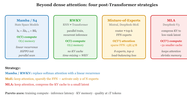
Section 3.5 covered variations on attention itself: positional schemes, sparse and linear attention, and the choice of normalization. This section looks at the next layer of innovation: architectures that step outside dense softmax attention. State space models replace quadratic attention with a linear recurrence. RWKV blends RNN inference with parallel training. Mixture-of-Experts keeps attention but routes each token through a tiny fraction of the FFN parameters. Multi-Head Latent Attention compresses the KV cache itself. The unifying theme is the same Pareto frontier of memory, compute, and quality, attacked from different angles.
Prerequisites
This section builds on the complete Transformer architecture from Section 3.1, the hands-on implementation from Section 3.3, and the attention and normalization variants from Section 3.5. The KV cache and inference-optimization themes (along with the survey of production architectures) are revisited later in the book.
3.8.1 Beyond Attention: State Space Models
State Space Models reveal that sequence modeling is fundamentally a problem of dynamical systems theory, a branch of mathematics shared by control engineering, signal processing, and physics. The continuous-time state equation dx/dt = Ax + Bu is the same formalism used to model electrical circuits, mechanical oscillators, and chemical reaction kinetics. The key insight from S4 and Mamba is that by carefully initializing the state matrix A using results from approximation theory (specifically, the HiPPO framework, which optimally compresses a continuous input history into a finite-dimensional state), you can build sequence models that rival Transformers on long-range tasks while maintaining linear time complexity. This cross-pollination from control theory to language modeling illustrates a broader pattern in science: mathematical structures that solve one problem often transfer surprisingly well to seemingly unrelated domains.
State Space Models borrow their mathematical framework from control theory, a field originally developed to stabilize rockets and autopilots. The idea that the same equations used to keep a spacecraft on course could also help a language model remember context across long documents is a beautifully unexpected connection.
State Space Models (SSMs) represent a fundamentally different approach to sequence modeling. Instead of computing pairwise attention between all tokens, SSMs process sequences through a linear recurrence with continuous-time dynamics. The key innovation is that this recurrence can be computed in O(T log T) time during training (using a parallel scan or convolution) while maintaining O(1) per-step cost during inference.
3.8.1.1 The S4 Foundation
S4 (Gu et al., 2022) models the mapping from input $u(t)$ to output $y(t)$ through a linear state-space equation:
After discretization with step size $\Delta$, this becomes a linear recurrence: $h_{t} = \bar{A}h_{t-1} + \bar{B}u_{t}$. The discrete recurrence can also be unrolled as a convolution (over the full sequence), enabling parallel training. S4's breakthrough was showing how to parameterize the matrix $A$ (using the HiPPO initialization) to capture long-range dependencies that RNNs struggle with.
3.8.1.2 Mamba: Selective State Spaces
Mamba (Gu and Dao, 2023) introduced selective state spaces, where the parameters B, C, and $\Delta$ are input-dependent (functions of the current token). This breaks the linear time-invariance that allows convolution-based training, but the authors developed a hardware-aware parallel scan algorithm that achieves efficient training on GPUs.
Mamba's advantages over Transformers:
- Linear time complexity in sequence length (vs. quadratic for attention)
- Constant memory during inference: no KV cache that grows with context
- Fast inference: each new token requires only a fixed-size state update
- Strong performance on tasks requiring long-range reasoning (up to millions of tokens)
Mamba's disadvantages:
- Cannot perform arbitrary lookback into the full context the way attention can; information must be compressed into the finite-dimensional state
- Harder to parallelize across the sequence dimension during training compared to attention
- Fewer mature optimization tools (no equivalent of FlashAttention yet for all SSM variants)
"O(T) beats O(T²), so Mamba must be strictly better than attention" is the most-repeated wrong reading of this section. A fixed-dimensional SSM state has finite capacity: once a fact is compressed into the state, retrieving it later is approximate. Attention can still pull out the exact token from 100K tokens ago, because the key-value pairs are stored verbatim. This is why benchmarks like the multi-needle-in-a-haystack consistently favor attention. Linear-time scaling is real, but the quality tradeoff at long context is non-trivial, which is why production stacks (Jamba, DeepSeek-V3) hybridize rather than replace.
Who: A research engineer at a legal AI startup exploring architectures for analyzing contracts up to 100,000 tokens long.
Situation: The startup's existing Transformer-based system truncated contracts to 8,192 tokens (the model's context limit), missing critical clauses in longer documents. They needed a model that could process full contracts without truncation.
Problem: Extending the Transformer's context to 128K tokens with standard attention would require quadratic memory, making it infeasible on their A100 GPUs. Even with FlashAttention, inference time scaled linearly with the square of the context length.
Dilemma: They evaluated three options: a Transformer with FlashAttention-2 and a 128K context window (expensive but proven), a pure Mamba model (linear scaling but less mature), or a hybrid architecture (Jamba-style, interleaving attention and SSM layers).
Decision: They chose the hybrid approach, using a Jamba-style architecture with one attention layer for every seven SSM layers. The attention layers provided exact retrieval for cross-referencing specific clauses, while the SSM layers efficiently processed the bulk of the document.
How: They fine-tuned the hybrid model on 5,000 annotated legal contracts, using the SSM layers for general comprehension and relying on the sparse attention layers to handle tasks requiring precise token-level lookback (e.g., "does evaluation metrics contradict softmax?").
Result: The hybrid model processed 100K-token contracts with 60% less GPU memory than a full-attention Transformer. Accuracy on clause extraction matched the Transformer baseline, while cross-reference detection (requiring long-range lookback) scored 91% vs. 78% for a pure Mamba model.
Lesson: Hybrid architectures that combine SSM efficiency with selective attention layers offer the best tradeoff for tasks requiring both long-context processing and precise information retrieval.
The success of hybrid architectures raises a natural question: are SSMs and attention really so different? Recent theoretical work suggests they may be closer than anyone expected.
3.8.1.3 Mamba-2 and the Connection to Attention
Mamba-2 (Dao and Gu, 2024) revealed a deep connection between SSMs and attention. The structured state space duality (SSD) framework shows that selective SSMs are equivalent to a form of structured masked attention, where the mask has a specific semiseparable structure. This unification opens the door to transferring optimization techniques between the two paradigms.
The Mamba-2 duality between SSMs and attention reveals something profound: all sequence models face the same fundamental tradeoff between memory and computation, just at different points on the Pareto frontier. Attention stores the entire history explicitly (the KV cache) and computes interactions on demand, like an open-book exam. SSMs compress history into a fixed-size state and must reconstruct what they need, like a closed-book exam where you memorized the material. This tradeoff echoes a classic result in computational complexity: the space-time tradeoff, where any computation can trade memory for processing time and vice versa. The convergence of SSMs and attention via the SSD framework suggests there may be a unified mathematical structure underlying all sequence models, just as statistical mechanics unifies different descriptions of the same physical system (microcanonical, canonical, grand canonical) as perspectives on the same underlying reality.
3.8.2 RWKV: Linear Attention as an RNN
RWKV (Peng et al., 2023) combines the training parallelism of Transformers with the inference efficiency of RNNs. It uses a variant of linear attention with time-dependent decay, formulated so that it can be computed either as a parallel attention-like operation (for training) or as a sequential RNN (for inference).
The core idea: replace softmax attention with a weighted sum using exponentially decaying weights:
Here $w$ is a learned decay factor (how quickly the model "forgets" past tokens) and $u$ is a bonus for the current token. This can be computed in O(T) during both training and inference. RWKV-6 and later versions add more sophisticated mechanisms (data-dependent linear interpolation, multi-scale decay) while maintaining linear complexity.
3.8.3 Mixture-of-Experts (MoE)
Mixture-of-Experts is an orthogonal scaling strategy: instead of making every layer wider, you create multiple "expert" sub-networks and route each token to only a few of them. This dramatically increases the total parameter count (and thus model capacity) while keeping the computation per token roughly constant.
The clearest way to see why MoE "multiplies capacity without multiplying compute" is to count parameters on a concrete dense FFN and then split it into experts. Take the original Transformer's FFN with $d_{\text{model}} = 512$ and $d_{\text{ff}} = 2048$. The two linear projections account for
Now split the hidden dimension $2048$ into $E = 16$ disjoint chunks of $128$ each, and turn each chunk into a separate expert FFN with its own narrow projections. Each expert has hidden width $128$, so its parameter count is
Sixteen such experts collectively hold $16 \cdot 131\text{K} \approx 2.1$M parameters, the same budget as the original dense FFN. The trick is the router: for any given token, only one expert (or a small top-$k$ subset) fires, so the active FLOPs per token are $1/16$th (or $k/16$th) of the dense FFN's cost. Multiply by an integer scaling factor: keep the per-expert width at $128$ but raise the expert count from $16$ to $128$. The total parameter pool grows to $128 \cdot 131\text{K} \approx 17$M (eight times the dense budget), yet a top-1 router still touches only $131\text{K}$ per token. That is the single arithmetic identity that powers Switch Transformer, Mixtral, and DeepSeek-V3: capacity (total params) decouples from compute (active params).
3.8.3.1 Architecture
The router (also called the gating network) is just one linear layer followed by a softmax over the expert dimension. For an input token vector $x \in \mathbb{R}^{d_{\text{model}}}$ and a router weight matrix $W_g \in \mathbb{R}^{d_{\text{model}} \times E}$, the per-expert gate score is
Sparse routing then keeps only the top-$k$ entries of $g(x)$ (typically $k = 1$ for Switch Transformer and Llama 4, $k = 2$ for Mixtral, $k = 6$ to $8$ for DeepSeek-V2/V3), re-normalizes those $k$ weights so they sum to one, and combines the chosen experts' outputs accordingly. A small ASCII sketch of the routed data flow follows; the dispatcher (the router box) is conceptually identical to the parcel-depot analogy below.
    token x (d_model)
            |
            v
   +----------------+        g(x) = softmax(x W_g)  in R^E
   |  router (W_g)  | -------------------------------+
   +----------------+                                |
            |                                        |
            v                                        v
       top-k indices                   gate weights g_top (k floats)
            |                                        |
   +--------+--------+----- ... -------+             |
   |        |        |                 |             |
   v        v        v                 v             |
  +---+   +---+   +---+              +---+           |
  |E1 |   |E2 |   |E3 |    ...       |EE |           |
  +---+   +---+   +---+              +---+           |
   |       |       |                   |             |
   v       v       v                   v             |
  out1   out2    out3                outE            |
   \       |        /                                |
    \      |       /                                 |
     \     |      /  weighted sum:                   |
      v    v     v   y = sum_{j in top-k} g_top[j] * E_{idx[j]}(x)
            y                                        |
            |<---------------------------------------+
            v
        next layer
Out of $E$ courier vans, only $k$ run for any given parcel; the rest sit idle for that token. The next token might pick a completely different subset of $k$ vans, so over a batch every expert sees enough traffic to keep training, provided the load-balancing loss does its job.
3.8.3.1.1 PyTorch Sketch
In a typical MoE Transformer, the FFN in each block is replaced by a set of $E$ expert FFNs plus a router (gating network). For each token, the router selects the top-$k$ experts (typically k=1 or k=2), and the token is processed only by those selected experts. The output is a weighted combination of the expert outputs.
from torch import nn
import torch
# Mixture-of-Experts FFN: a learned router selects top-k experts per token.
# Only the selected experts run, keeping compute constant as total params grow.
class MoELayer(nn.Module):
    """Mixture-of-Experts feed-forward layer."""
    def __init__(self, d_model, d_ff, n_experts, top_k=2):
        super().__init__()
        self.n_experts = n_experts
        self.top_k = top_k
        # Router: maps d_model -> n_experts (logits for each expert)
        self.router = nn.Linear(d_model, n_experts, bias=False)
        # Expert FFNs
        self.experts = nn.ModuleList([
            nn.Sequential(
            nn.Linear(d_model, d_ff, bias=False),
            nn.SiLU(),
            nn.Linear(d_ff, d_model, bias=False),
            )
            for _ in range(n_experts)
            ])
    def forward(self, x):
        B, T, C = x.shape
        x_flat = x.view(-1, C) # (B*T, C)
        # Compute routing weights
        router_logits = self.router(x_flat) # (B*T, n_experts)
        weights, indices = torch.topk(router_logits, self.top_k, dim=-1)
        weights = torch.softmax(weights, dim=-1) # normalize top-k
        # Dispatch tokens to experts and combine results
        output = torch.zeros_like(x_flat)
        for k in range(self.top_k):
            expert_idx = indices[:, k] # (B*T,)
            weight = weights[:, k].unsqueeze(-1) # (B*T, 1)
            for e in range(self.n_experts):
                mask = (expert_idx == e)
                if mask.any():
                    expert_input = x_flat[mask]
                    expert_output = self.experts[e](expert_input)
                    output[mask] += weight[mask] * expert_output
                    return output.view(B, T, C)
A naive router tends to collapse: it learns to send all tokens to the same few experts, leaving most experts unused. To prevent this, MoE models add an auxiliary load-balancing loss that penalizes imbalanced expert utilization. The balancing loss encourages the router to distribute tokens roughly equally across experts. Mixtral, Switch Transformer, and GShard all use variants of this technique.
Picture the MoE layer as a parcel depot at rush hour. Each token is a parcel arriving at the dispatcher's desk; the router is the dispatcher; the $E$ experts are courier vans waiting in numbered bays. The dispatcher reads the parcel's label (the token representation) and assigns it to the two vans best suited to deliver it (top-$k$ routing). The vans process only the parcels they receive, so doubling the number of vans doubles total capacity without doubling each parcel's delivery time. That is the entire scaling argument for MoE in one image.
Left alone, dispatchers develop favorites. They funnel almost every parcel to vans 1 and 2 because those vans return early reward (lower loss), while vans 3 through 8 idle in the lot, never improving, slowly becoming useless. The auxiliary loss is the depot manager standing behind the dispatcher with a clipboard, tallying how many parcels went to each bay and how confidently the dispatcher leaned toward each van. The term $\alpha \cdot E \cdot \sum_i f_i \cdot p_i$ penalizes the dispatcher whenever the fraction of parcels sent to van $i$ (hard statistic $f_i$) and the gate's enthusiasm for van $i$ (smooth statistic $p_i$) both point at the same bay, nudging the dispatcher to spread work evenly so every van earns its keep.
Algorithm: Sparse Mixture-of-Experts FFN
Input:  token representation x in R^{B x T x d}, E experts {f_1,..,f_E}, top_k = k
Output: y in R^{B x T x d}, plus auxiliary load-balancing loss L_aux

  // 1. Router scores every expert
  g := softmax(x @ W_r)                         // (B, T, E), W_r in R^{d x E}

  // 2. Select top-k experts per token; re-normalize their gates
  (g_top, idx) := topk(g, k, axis = -1)         // each (B, T, k)
  g_top := g_top / sum(g_top, axis = -1, keepdims = True)

  // 3. Dispatch each token to its chosen experts, combine outputs
  y := 0
  For j = 1..k:
      e := idx[..., j]                          // chosen expert index per token
      y := y + g_top[..., j] * f_{e}(x)         // gated expert output

  // 4. Switch Transformer auxiliary loss (Fedus et al., 2021)
  //    f_i = fraction of tokens routed to expert i
  //    p_i = mean gate probability for expert i across the batch
  f := one_hot(idx, E).mean(axis = (B, T, k))   // dispatch fraction per expert
  p := g.mean(axis = (B, T))                    // mean router probability per expert
  L_aux := E * alpha * sum_i (f_i * p_i)        // alpha ~ 0.01

  Return y, L_aux

Why this loss balances? p_i is differentiable in W_r; f_i is not, but in the product f_i * p_i,
gradients pushed by alpha lower p_i precisely for over-used experts, encouraging the router to
spread mass uniformly. A perfectly balanced router yields E * sum_i (1/E)^2 = 1.
Sources: Shazeer et al., "Outrageously Large Neural Networks: The Sparsely-Gated Mixture-of-Experts Layer" (arXiv:1701.06538, ICLR 2017) introduced the top-k gating mechanism; Fedus et al., "Switch Transformer" (arXiv:2101.03961, 2021) defined the modern $f_i \cdot p_i$ auxiliary loss used in Mixtral, DeepSeek-MoE, and Llama 4. DeepSeek-V3 (2024) further introduced auxiliary-loss-free balancing via per-expert bias updates, sidestepping the gradient-routing trade-off entirely.
3.8.3.2 Notable MoE Models
| Model | Total Params | Active Params | Experts | Top-k |
|---|---|---|---|---|
| Switch Transformer | 1.6T | ~100B | 128 | 1 |
| Mixtral 8x7B | 46.7B | 12.9B | 8 | 2 |
| Mixtral 8x22B | 176B | 39B | 8 | 2 |
| DeepSeek-V2 | 236B | 21B | 160 | 6 |
| Qwen2-MoE | 57B | 14.3B | 64 | 8 (shared + routed) |
| DeepSeek-V3 | 671B | 37B | 256 | 8 |
| Llama 4 Maverick | 400B | 17B | 128 | Top-1 routed |
| Llama 4 Scout | 109B | 17B | 16 | Top-1 routed |
The key insight: a 46.7B parameter MoE model (Mixtral 8x7B) can match or exceed a dense 70B model in quality while using only 12.9B parameters of computation per token. This means it runs at roughly the speed of a 13B dense model despite having the knowledge capacity of a much larger one.
The MoE table above illustrates a crucial point: Mixtral 8x7B has 46.7B total parameters but activates only 12.9B per token, yet it matches dense 70B models on many benchmarks. Parameter count alone is a poor predictor of model quality. What matters is the effective computation per token (active parameters), the training data quality and quantity, and the architectural efficiency. A well-trained 7B dense model can outperform a poorly trained 70B model. When comparing models, always ask: how many parameters are active per forward pass? How much training data was used? What is the training compute budget (FLOPs)? These factors are more predictive than raw parameter counts.
The 2024 and 2025 releases confirm MoE as the dominant scaling paradigm. DeepSeek-V3 (December 2024) pushed the frontier with 671B total parameters and 256 fine-grained experts, using auxiliary-loss-free load balancing and multi-token prediction heads. Despite its enormous capacity, only 37B parameters activate per token, keeping inference costs manageable. Meta's Llama 4 family (2025) completed Meta's own transition from dense to MoE: Llama 4 Scout (109B total, 16 experts) and Llama 4 Maverick (400B total, 128 experts) both use top-1 expert routing, meaning each token activates a single expert plus shared parameters. Both Llama 4 variants are natively multimodal, processing text and images in a unified architecture. The trend is clear: leading labs have converged on MoE as the way to scale model knowledge without proportionally scaling inference cost.
3.8.3.3 Routing Strategies, Named
The MoE literature uses several near-synonymous names for routing strategies; it helps to put them on one chip-sheet:
- Top-k routing (also called KeepTopK in Shazeer et al., 2017): keep the $k$ experts with the highest gate scores per token, re-normalize their weights, dispatch. $k = 2$ is the historical default and the choice in Mixtral.
- Switch routing (Fedus, Zoph, Shazeer 2021): the $k = 1$ special case. Each token is sent to exactly one expert. Conceptually a "hard router". Used by Switch Transformer and by both Llama 4 variants.
- Noisy top-k: Gaussian noise is added to the router logits before the softmax during training to encourage exploration of under-used experts. Drops away at inference.
- Soft / dense routing: all $E$ experts run, but their outputs are mixed with the full softmax weights. Used in some research papers (e.g., Soft-MoE 2023) but rare in production because the FLOPs-per-token grow with $E$.
- Expert Choice routing (Zhou et al., 2022): invert the dispatch direction. Each expert picks its top-$N$ tokens instead of each token picking its top-$k$ experts. Guarantees perfect load balance without an auxiliary loss but breaks autoregressive causality and so is mostly used for encoder-only pretraining.
- Auxiliary-loss-free routing (DeepSeek-V3, 2024): maintain a per-expert bias term that the trainer adjusts after each step to nudge under-used experts toward selection, sidestepping the gradient-versus-routing trade-off baked into the Switch-style $\alpha \cdot E \cdot \sum f_i p_i$ loss.
3.8.3.4 The GShard - Switch - Mixtral - DeepSeek Lineage
MoE went from research curiosity to frontier-default in roughly six years. The lineage is worth following because each step solved a specific blocker.
- Sparsely-Gated MoE (Shazeer et al., 2017) introduced the modern formulation: a top-$k$ gating network on top of many small expert FFNs, trained jointly with a load-balancing auxiliary loss. Demonstrated on machine translation with up to 137B parameters at a time when dense state of the art was ~1B.
- GShard (Lepikhin et al., 2020) brought MoE to large-scale multilingual machine translation (600B parameters, 2048 experts) and introduced the practical engineering: token-to-expert dispatching across TPU pods, capacity factor to bound per-expert tokens, and the all-to-all collective that is now the canonical MoE communication primitive.
- Switch Transformer (Fedus et al., 2021) simplified routing to top-1, demonstrated that the $f_i \cdot p_i$ auxiliary loss is sufficient for balance, and scaled to 1.6T parameters. The Switch paper's clean ablations on capacity factor, expert count, and routing-loss coefficient are the source of most modern defaults.
- GLaM (Du et al., 2022), ST-MoE (Zoph et al., 2022), and NLLB-MoE (Costa-jussa et al., 2022) filled in the recipe: router z-loss for numerical stability, fine-tuning-time freezing tricks, and the demonstration that MoE quality scales similarly to dense quality per active parameter.
- Mixtral 8x7B (Jiang et al., 2024) made MoE practical for the open-source community. Eight experts, top-2 routing, 47B total / 13B active parameters, Apache-2.0 weights. Quality matched or exceeded dense LLaMA-2-70B at one-third the inference cost.
- DeepSeek-V2 (2024) and DeepSeek-V3 (December 2024) pushed the design toward many fine-grained experts (256 in V3) with auxiliary-loss-free routing and shared "always-on" experts for common knowledge. V3's 671B total / 37B active configuration is the current public state of the art and the architecture behind DeepSeek-R1's reasoning successes.
- Llama 4 Scout and Maverick (Meta, 2025) completed the transition: Meta's flagship line moved from dense to top-1 MoE for both compute economics and multimodal scaling reasons.
The common thread is unchanged from Shazeer 2017: decouple total parameters (where knowledge lives) from active parameters (where the FLOP bill is paid), pay the engineering cost of an all-to-all dispatch, and accept that the router will need careful balancing to keep every expert useful.
3.8.4 Gated Attention and Gated Linear Units
The concept of gating (element-wise multiplication of two parallel pathways) has become ubiquitous in modern Transformers, appearing in both the FFN and the attention mechanism.
3.8.4.1 Gated FFN Variants
The standard ReLU FFN computes ReLU(xW1)W2. Gated variants split
the first projection into two branches and multiply them:
- GLU (Dauphin et al., 2017):
(xW1 ⊙ σ(xWgate))W2 - GEGLU: Replace σ with GELU activation
- SwiGLU (Shazeer, 2020): Replace σ with SiLU (Swish). This is the standard in LLaMA, PaLM, Mistral, Gemma
Why does gating help? The gate branch learns to selectively amplify or suppress features produced by the value branch. This provides a richer form of nonlinearity than a single activation function and consistently improves performance at a given compute budget.
3.8.4.2 Gated Attention Units
GAU (Hua et al., 2022) applies the gating principle to attention itself. Instead of the standard residual attention pattern, GAU computes:
where U is a gating signal derived from the input, and V is the value signal. This allows single-head attention to be competitive with multi-head attention, since the gate provides the diversity that multiple heads normally provide. GAU reduces both the number of attention heads needed and the overall parameter count.
3.8.5 Multi-Head Latent Attention (MLA)
Multi-Head Latent Attention (DeepSeek-V2, 2024) addresses the KV cache bottleneck through a different lens than GQA. Instead of sharing KV heads across groups, MLA compresses the keys and values into a low-dimensional latent space before caching.
3.8.5.1 How MLA Works
In standard attention, we cache the full K and V tensors of shape $(T, n_{heads}, d_k)$. MLA instead caches a compressed representation $c_{KV}$ of shape $(T, d_c)$ where $d_c << n_{heads} \times d_k$. The full K and V are reconstructed from the compressed representation when needed:
The compression ratio can be 4x to 16x, dramatically reducing the KV cache memory. The decompression matrices $W_{UK}$ and $W_{UV}$ are small and fast to apply. DeepSeek-V2 reports comparable quality to standard multi-head attention while reducing KV cache memory by 93%.
There is a progression of techniques for reducing KV cache size: standard MHA (full cache) → GQA (share KV across groups, ~4x reduction) → MQA (single KV, ~32x reduction) → MLA (compressed latent, 4x to 16x with less quality loss than MQA). Each trades off differently between cache size, computation, and model quality.
3.8.6 Putting It All Together: Modern LLM Recipes
No production LLM uses a single technique in isolation. Here is how several prominent models combine the building blocks discussed across Section 3.5 (attention & normalization variants) and this section (SSMs, MoE, MLA):
| Model | Architecture | Position Enc. | Attention | FFN | Special |
|---|---|---|---|---|---|
| Llama-3 | Decoder-only | RoPE | GQA | SwiGLU | Pre-LN (RMSNorm) |
| Mistral 7B | Decoder-only | RoPE | GQA + sliding window | SwiGLU | Pre-LN (RMSNorm) |
| Mixtral 8x7B | Decoder-only MoE | RoPE | GQA + sliding window | SwiGLU MoE (8 experts) | Top-2 routing |
| DeepSeek-V2 | Decoder-only MoE | RoPE (YaRN) | MLA | MoE (160 experts) | Top-6 routing, shared experts |
| Jamba | Hybrid SSM+Attn | RoPE (Attn layers) | GQA (some layers) | SwiGLU MoE | Mamba + Attention interleaved |
| Gemma 2 | Decoder-only | RoPE | GQA + local/global | GeGLU | Alternating local/global attention |
- State Space Models (Mamba, S4) offer linear-time sequence processing by replacing pairwise attention with a recurrent linear dynamical system; the cost is lossy compression of the context into a finite-size state.
- Mamba-2 reveals that selective SSMs are equivalent to a form of structured masked attention, suggesting SSMs and attention occupy different points on the same memory-compute Pareto frontier.
- Hybrid SSM+attention architectures (Jamba, Zamba, Samba) interleave layers from both paradigms to get efficient long-context processing plus selective exact retrieval.
- RWKV combines the parallel training of attention with the constant-time inference of RNNs by using exponentially-decayed linear attention with a recurrent reformulation.
- Mixture-of-Experts dramatically increases model capacity (total parameters) while keeping per-token compute roughly constant by routing each token to only the top-k of E experts; load-balancing auxiliary loss is essential to prevent router collapse.
- Active parameters (not total parameters) determine inference latency; memory is determined by total parameters. This decoupling is the entire reason MoE is interesting.
- Gating (SwiGLU, GAU) is ubiquitous in modern architectures, providing richer nonlinearities than a single activation can.
- Multi-Head Latent Attention (MLA) compresses the KV cache into a low-dimensional latent vector, sitting between full MHA and aggressive MQA on the quality vs. memory curve.
- Frontier 2024 to 2026 LLMs (DeepSeek-V3, Llama 4, Mixtral, Gemma 2, Jamba) combine RoPE, GQA or MLA, SwiGLU, Pre-LN with RMSNorm, and, increasingly, MoE; the recipe is fairly standardized across labs.
Show Answer
Show Answer
Show Answer
Show Answer
Exercises
Mixtral 8x7B has 8 experts per layer, top-2 routing, and reports 46.7B total but 12.9B active parameters. (a) What is the per-token compute reduction relative to a dense model with 46.7B parameters? (b) If you increased to top-4 routing (keeping 8 experts), what would active parameters become and what tradeoff are you making? (c) Explain why "active params" matters for latency but "total params" matters for memory.
Answer Sketch
(a) Active is 12.9/46.7 = 28% of total, so per-token compute is roughly 28% of a dense 46.7B model: a 3.6x speedup. Each token only flows through 2 of 8 expert FFNs plus shared attention. (b) Top-4: roughly half the FFN parameters become active, so active rises to roughly 21B (FFN doubles, attention/embeddings unchanged). Tradeoff: more compute per token (slower) for potentially better quality (more expert mixing). Empirically the gain is modest because routing already finds the most relevant experts at top-2. (c) Latency: each forward pass only computes the active experts, so wall-clock time scales with active params. Memory: all 8 experts must be in GPU memory because we don't know which experts will be needed for the next token; we cannot dynamically swap experts in/out without massive PCIe overhead. So memory scales with total params, latency with active params, which is the entire reason MoE is interesting.
The chapter notes that without load-balancing loss, MoE routers tend to collapse and send all tokens to a few experts. (a) Why does this collapse happen mathematically? (b) Describe what training metrics would alert you to router collapse during a training run. (c) The auxiliary load-balancing loss has weight α typically 0.01 to 0.1; what goes wrong if α is too high or too low?
Answer Sketch
(a) The router has a winner-take-all dynamic: at initialization, one expert is slightly more activated by chance; gradient descent makes the router send slightly more tokens to it; that expert trains faster (more data) and becomes better; the router learns to send even more tokens to it; etc. This is a positive-feedback loop that culminates in 1-2 experts handling all tokens. (b) Metrics: per-expert token counts (should be roughly uniform); router entropy (should be high, close to $\log(\text{n\_experts})$); per-expert gradient norms (collapsed experts have small or zero gradients). Mixtral-style monitoring computes the "expert utilization variance" and alerts above a threshold. (c) Too high: the auxiliary loss dominates the language modeling loss, forcing uniform routing regardless of token content; the router becomes random, defeating the purpose of MoE. Too low: insufficient regularization, collapse occurs anyway. The 0.01 sweet spot reflects roughly a 1% perturbation to the main loss.
You are evaluating two models on a 100K-token document QA task: a Transformer with FlashAttention-2, and a pure Mamba model. (a) Which model is likely faster at inference, and why? (b) Which model is likely more accurate on a question that requires retrieving an exact phrase from token position 73,421, and why? (c) What hybrid architecture would you design to get both, and what is the simplest 80/20 split that captures most of the benefit?
Answer Sketch
(a) Mamba: O(T) inference cost per generated token vs. O(T) for cached attention (but with smaller constants and no growing KV cache). Crucially, Mamba uses constant memory for state, while attention's KV cache at 100K tokens is multi-GB even with GQA. (b) The Transformer: exact retrieval is exactly what attention is good at; Mamba must reconstruct the phrase from a fixed-size state and is likely to blur or lose precise tokens. (c) A Jamba-style hybrid with roughly one attention layer per seven SSM layers. The SSM layers carry the bulk of the computation cheaply; the few attention layers provide the precise lookback needed for retrieval-heavy questions. Empirically this captures most of the long-context advantage of pure attention at a fraction of the cost.
A team is choosing between GQA (8 KV groups, n_heads=64, d_k=128) and MLA (latent dim d_c=512) for a 70B-class model at 32K context in FP16. (a) Compute the KV cache size per layer for each. (b) Which is more memory efficient? (c) What additional compute cost does MLA pay at attention time that GQA does not, and why is it usually worth it?
Answer Sketch
(a) GQA per layer: 2 (K+V) × 32768 × 8 × 128 × 2 bytes = 134 MB. MLA per layer: 32768 × 512 × 2 bytes = 32 MB (one cached latent, not separate K and V). (b) MLA is roughly 4x smaller per layer, so over 80 layers MLA stores ~2.6 GB vs. ~10.7 GB for GQA. (c) MLA must reconstruct K and V from the cached latent at every attention step (matmuls with W_UK and W_UV). This is extra FLOPs but the matrices are small and the reconstruction can be batched. The tradeoff is usually worth it for long-context decoding because memory bandwidth (loading the KV cache) is the inference bottleneck, not compute; MLA shrinks the bandwidth-bound term at the cost of a small compute-bound term.
Architecture innovation is accelerating. DeepSeek-V3 (2024) combines multi-head latent attention (MLA) with DeepSeekMoE for efficient 671B-parameter models. Mamba-2 and Jamba-1.5 demonstrate that hybrid state-space/attention architectures can match pure Transformer performance. xLSTM (Beck et al., 2024) revisits the LSTM with exponential gating and matrix memory. Ring Attention (Liu et al., 2023) enables million-token contexts by distributing attention across devices, while MoE models (Mixtral, Grok) activate only a fraction of parameters per token.
What's Next?
In the next chapter, Chapter 4: Decoding Strategies and Text Generation, we shift from architecture to generation, exploring the decoding strategies that turn model outputs into coherent text. The frontier architectures touched on here are revisited in depth in Chapter 75: Frontier Architectures.