"FSDP makes parameters fit; tensor parallelism makes activations fit. Two all-reduces per block, eight GPUs per node, and the NVLink fanout decides where it stops."
Tensor, Shard-Counting AI Agent
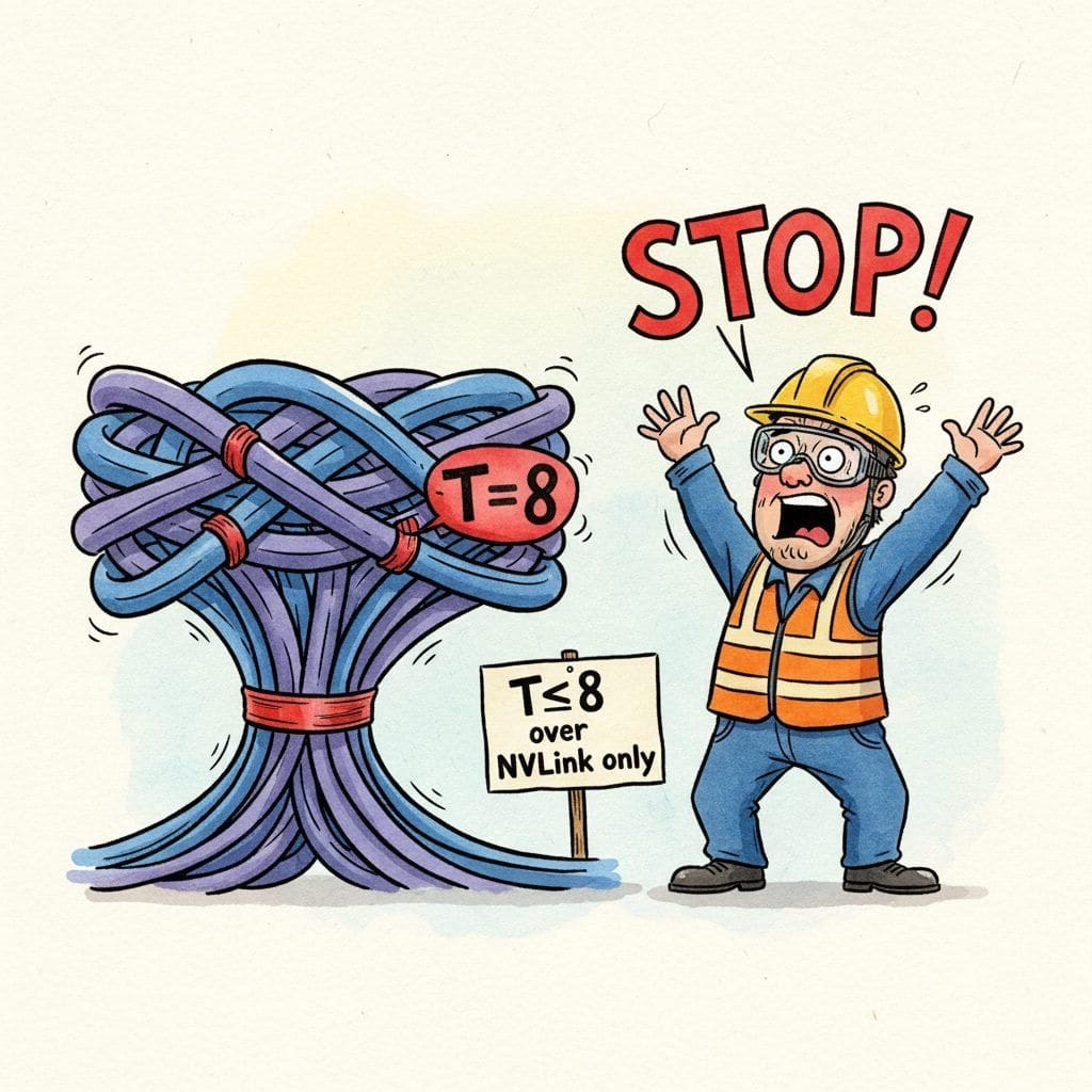
FSDP shards across the data dimension; tensor parallelism shards within a layer. Megatron-LM (Shoeybi et al., 2019) showed that a transformer's MLP and attention blocks can be partitioned across $T$ GPUs with exactly two all-reduces per transformer block: one after the MLP down-projection, one after the attention output projection. Sequence parallelism extends this to dropout and layer-norm so activation memory also shards. The combination is what every Megatron / DeepSpeed / NeMo frontier training stack runs internally. Tensor parallelism is bandwidth-hungry: it works inside a node on NVLink and dies on InfiniBand. The 8-way tensor-parallel limit you see everywhere is the NVLink fanout, not a software choice.
Prerequisites
This section assumes familiarity with ZeRO and FSDP sharding from Section 59.2 and with data-parallel training fundamentals from Section 59.1. Familiarity with multi-head attention internals from Section 2.2 helps when reading the MLP-and-attention partition discussion.
59.3.1 Why Not Just FSDP?
Megatron-LM was named after the Transformers villain because NVIDIA's Mohammad Shoeybi thought "we are sharding the Transformer, so the name should sound like a robot that has been cut into pieces". The codebase still ships an ASCII-art Megatron banner that prints when you launch a training job, which has survived three major refactors and a complete API rewrite.
FSDP makes parameters fit. It does not make activations fit. Activation memory scales with batch size, sequence length, and the number of layers; for a 70B model with $B \cdot L = 8 \cdot 8192 = 65\text{k}$ tokens, the per-rank activation working set can reach 200 GB even after checkpointing. FSDP replicates this full activation set on every rank because, from FSDP's perspective, each rank is running the full model on its own data slice.
Tensor parallelism solves this by sharding the computation, not just the storage. Each rank performs a sliver of every matmul; both the parameters and the activations are intrinsically $T\times$ smaller on each rank. The penalty is one extra collective per matmul, but with NVLink that is a tiny fraction of the matmul wall-time.
59.3.2 Column-Parallel and Row-Parallel Matmul
Tensor parallelism rests on two ways to split a matrix multiplication $Y = XW$ where $X \in \mathbb{R}^{B \times d_{\text{in}}}$ and $W \in \mathbb{R}^{d_{\text{in}} \times d_{\text{out}}}$.
59.3.2.1 Column-Parallel
Split $W$ along its columns:
Each rank $t$ holds $W^{(t)}$ and computes $Y^{(t)} = X W^{(t)}$. The full output is the column-wise concatenation $Y = [Y^{(1)} \mid Y^{(2)} \mid \cdots \mid Y^{(T)}]$, with each rank owning its slice. No forward communication is required when the input $X$ is replicated; the backward pass requires an all-reduce on $\partial L / \partial X$ because each rank computed a partial gradient. We write this as the identity-then-all-reduce pattern, often called $f$ in the Megatron literature: $f$ is identity in forward, all-reduce in backward.
59.3.2.2 Row-Parallel
Split $W$ along its rows:
Now each rank's input must be the corresponding slice: $X^{(t)} \in \mathbb{R}^{B \times d_{\text{in}}/T}$. Each rank computes $Y^{(t)} = X^{(t)} W^{(t)}$, and the partial outputs sum to the full output: $Y = \sum_{t} Y^{(t)}$. The forward pass requires an all-reduce across ranks; the backward pass is identity. This is the all-reduce-then-identity pattern, the $g$ function: $g$ is all-reduce in forward, identity in backward.
59.3.2.3 The Key Trick: Pair Them
A column-parallel matmul leaves the output sharded across ranks. A row-parallel matmul takes a sharded input. So two consecutive matmuls can be pipelined with only one all-reduce between them, by choosing the first column-parallel and the second row-parallel. The MLP and attention blocks of a transformer are exactly this pattern.
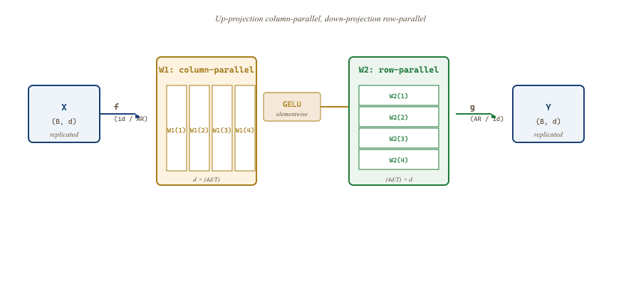
g all-reduces the partial sums (W2 output) so every rank receives the full activation, and on the backward pass f all-reduces the partial gradients so every rank receives the full $\partial L / \partial X$.59.3.3 The MLP Block in Detail
The transformer FFN is $Y = \text{GELU}(X W_1) W_2$ with $W_1 \in \mathbb{R}^{d \times 4d}$ and $W_2 \in \mathbb{R}^{4d \times d}$. Megatron's recipe:
Plug in Llama-3 70B's actual dimensions: $d = 8192$, $4d = 28672$, batch $B = 4$ sequences of length 8192. On 8 H100s with $T = 8$ tensor parallelism, the column-parallel $W_1$ shards into 8 slices of shape $8192 \times 3584$ per rank. The intermediate activation between $W_1$ and $W_2$ is $(4, 8192, 3584)$ per rank, roughly 470 MB in bf16, instead of $(4, 8192, 28672)$ at 3.7 GB on a single device. That is the 8x activation memory saving the section claims, but in concrete megabytes you can compare against the H100's 80 GB. The single all-reduce moves $(4, 8192, 8192)$ activations, 512 MB in bf16, across NVLink at 900 GB/s, costing 0.6 ms per MLP block. Across 80 layers, that is 48 ms per forward pass, less than 5 percent of the typical step time on this configuration. Tensor parallelism trades a 0.6 ms all-reduce per block for a 3.2 GB activation memory saving per rank: cheap enough that nobody trains 70B without it.
- $W_1$ column-parallel: rank $t$ holds columns $[(t-1) \cdot 4d/T : t \cdot 4d/T]$. Input $X$ is replicated on every rank (no input comm). Output $Z^{(t)} = X W_1^{(t)}$ has shape $(B, 4d/T)$, partitioned across the hidden dimension.
- GELU is elementwise, so it runs locally on each rank's sharded $Z^{(t)}$.
- $W_2$ row-parallel: rank $t$ holds rows $[(t-1) \cdot 4d/T : t \cdot 4d/T]$. The input is already sharded (the GELU output), so each rank computes $Y^{(t)} = \text{GELU}(Z^{(t)}) W_2^{(t)}$, a partial sum of shape $(B, d)$.
- All-reduce across ranks: $Y = \sum_t Y^{(t)}$. Every rank now holds the full output.
One all-reduce, one matmul pair. The activation memory between $W_1$ and $W_2$ is $(B, 4d/T)$ per rank instead of $(B, 4d)$ on a single device: a $T\times$ saving on the largest intermediate of the MLP.
59.3.4 The Attention Block in Detail
Multi-head attention splits naturally along the head dimension. With $H$ heads of dimension $d_h$ where $H \cdot d_h = d$:
- QKV projection $W_{QKV} \in \mathbb{R}^{d \times 3d}$ is column-parallel; each rank holds $3 d_h \cdot H / T$ output columns, which is $H/T$ heads' worth of Q, K, V each.
- Attention itself runs locally on each rank because the heads are independent: rank $t$ computes attention on its $H/T$ heads with no cross-rank communication. This is the key insight: heads are already parallel along the right axis.
- Output projection $W_O \in \mathbb{R}^{d \times d}$ is row-parallel: each rank holds rows corresponding to its head outputs.
- All-reduce at the end of the row-parallel projection, mirroring the MLP.
So an attention block also costs exactly one all-reduce. A whole transformer block (attention + MLP) is two all-reduces. For a 96-layer model with $T=8$, that is 192 NVLink all-reduces per step on the forward pass plus 192 on the backward. Each all-reduce is a few microseconds on NVSwitch, so even at $T=8$ tensor parallelism the per-step communication is bounded by single-digit milliseconds.
59.3.4.1 Multi-Query and Grouped-Query Attention
Modern attention variants like multi-query attention (MQA, 1 KV head shared by all Q heads) and grouped-query attention (GQA, $G$ KV heads, each shared by $H/G$ Q heads) interact with tensor parallelism. The Q projection always shards normally; the K and V projections must respect the smaller head count. Llama-3 70B uses GQA with $G=8$ and $H=64$; with $T=8$ TP, each rank gets exactly one KV head and eight Q heads. This alignment is no accident: model architects pick KV head counts as multiples of the planned tensor-parallel degree, and tensor-parallel degree is chosen to match GQA group count.
The reason tensor parallelism is cheap for transformers is that multi-head attention already partitions the computation: $H$ heads are intrinsically independent. Splitting them across $T$ ranks is mechanical (no extra reductions inside attention). The only synchronization is at the output projection, which is the same all-reduce you would do for the MLP. Tensor parallelism is the answer to "where does the natural symmetry of the transformer want to be sharded?".
59.3.5 A Toy Tensor-Parallel Matmul
To make the mechanics crystal clear, here is a minimal PyTorch implementation of a column-parallel linear followed by a row-parallel linear, which together form one Megatron-style MLP. The pattern in production code (Megatron-LM, NeMo, vLLM serving) is identical; this strips it to its essentials.
# tp_minimal.py: torchrun --nproc_per_node=4 tp_minimal.py
import os, math, torch
import torch.distributed as dist
import torch.nn as nn

class ColumnParallelLinear(nn.Module):
    """Y = X W where W is sharded along its output (column) dim across ranks."""
    def __init__(self, in_features, out_features, world_size, rank):
        super().__init__()
        assert out_features % world_size == 0, "out_features must divide world_size"
        self.out_per_rank = out_features // world_size
        # Each rank owns a slice of the weight matrix.
        self.weight = nn.Parameter(
            torch.empty(self.out_per_rank, in_features, device="cuda")
        )
        nn.init.kaiming_uniform_(self.weight, a=math.sqrt(5))

    def forward(self, x):
        # Input is replicated; output is sharded along columns.
        # Backward will need an all-reduce on grad_x (handled by hook below).
        return _CopyToTPRegion.apply(x) @ self.weight.t()

class RowParallelLinear(nn.Module):
    """Y = X W where W is sharded along its input (row) dim across ranks."""
    def __init__(self, in_features, out_features, world_size, rank):
        super().__init__()
        assert in_features % world_size == 0
        self.in_per_rank = in_features // world_size
        self.weight = nn.Parameter(
            torch.empty(out_features, self.in_per_rank, device="cuda")
        )
        nn.init.kaiming_uniform_(self.weight, a=math.sqrt(5))

    def forward(self, x):
        # Input is sharded along last dim (matching col-parallel output).
        partial = x @ self.weight.t()
        # All-reduce sums partials -> full Y on every rank.
        return _AllReduceFromTPRegion.apply(partial)

# --- The f and g functions: identity / all-reduce on opposite passes. ---
class _CopyToTPRegion(torch.autograd.Function):
    @staticmethod
    def forward(ctx, x): return x                # identity
    @staticmethod
    def backward(ctx, g):
        dist.all_reduce(g)                       # sum partial gradients
        return g

class _AllReduceFromTPRegion(torch.autograd.Function):
    @staticmethod
    def forward(ctx, x):
        dist.all_reduce(x)                       # sum partial outputs
        return x
    @staticmethod
    def backward(ctx, g): return g               # identity

# --- A two-layer Megatron-style MLP ---
class TPMLP(nn.Module):
    def __init__(self, d, world_size, rank):
        super().__init__()
        self.up   = ColumnParallelLinear(d, 4*d, world_size, rank)
        self.down = RowParallelLinear(4*d, d, world_size, rank)
    def forward(self, x):
        return self.down(torch.nn.functional.gelu(self.up(x)))

if __name__ == "__main__":
    dist.init_process_group(backend="nccl")
    rank, world_size = dist.get_rank(), dist.get_world_size()
    torch.cuda.set_device(rank)

    mlp = TPMLP(d=4096, world_size=world_size, rank=rank)
    x = torch.randn(8, 1024, 4096, device="cuda")
    y = mlp(x)            # full y on every rank, with only one all-reduce per pass
    y.sum().backward()    # one all-reduce on grad_x

    dist.destroy_process_group()
_CopyToTPRegion ($f$ in Megatron's notation) and _AllReduceFromTPRegion ($g$) install the right collectives on the right pass. Production code uses Megatron's ColumnParallelLinear and RowParallelLinear which add bias handling, async comm, and fused kernels, but the pattern above is the entire idea.Never ship the from-scratch MLP above. megatron-core (NVIDIA, 2023+) is the production-grade slim of Megatron-LM that exposes ColumnParallelLinear, RowParallelLinear, VocabParallelEmbedding, and VocabParallelCrossEntropy as drop-in modules with async comm, fused bias handling, sequence-parallel support, and matching backward kernels. It is the same kernel set vLLM and NeMo use under the hood, and is the canonical answer when the warning above ("custom code silently produces wrong gradients") applies.
Show code
pip install megatron-core
import torch
from megatron.core import parallel_state
from megatron.core.tensor_parallel import (
    ColumnParallelLinear, RowParallelLinear,
)

parallel_state.initialize_model_parallel(tensor_model_parallel_size=8)

up = ColumnParallelLinear(d, 4 * d, bias=False, gather_output=False)
down = RowParallelLinear(4 * d, d, bias=False, input_is_parallel=True)

# forward pass: one all-reduce, identical to Code Fragment 59.3.1
h, _ = up(x)
y, _ = down(torch.nn.functional.gelu(h))parallel_state.initialize_model_parallel(tensor_model_parallel_size=T, pipeline_model_parallel_size=P) to compose with pipeline parallelism (Section 59.4) without rewriting the model.59.3.6 Sequence Parallelism: The FSDP Trick
Tensor parallelism shards the parameters and the matmul activations. But it leaves three operations replicated: dropout, layer-norm, and the residual add. Each of these holds an activation of shape $(B, L, d)$ on every rank. For a 70B model with $L=8192$, $d=8192$, $B=8$ in BF16, that is about $4.3$ GB per layer per rank, replicated $T$ times for no reason.
Sequence parallelism (Korthikanti et al., 2022) recognizes that this replication is wasteful: layer-norm and dropout are elementwise (sequence-independent), so they can be sharded along the sequence dimension just as the MLP is sharded along the hidden dimension. The two are composable: alternating between sequence-sharded and hidden-sharded activations across the layer.
The trick that makes this practical is the algebraic identity all-reduce = reduce-scatter + all-gather. Rather than an all-reduce at the MLP output (which materializes the full output on every rank), you do:
- Reduce-scatter after the row-parallel matmul: each rank ends up with $1/T$ of the output along the sequence dimension.
- Run layer-norm and dropout on the sequence-sharded activation. Memory drops by $T\times$.
- All-gather before the next attention block's input projection, which expects a full $(B, L, d)$ input.
Total wire bytes are the same as the original all-reduce; the working memory for the in-between operations is $T\times$ smaller. For an 8-way tensor parallel run on Llama-70B, sequence parallelism saves roughly 30 GB of activation memory per rank, which is the difference between fitting and not fitting at long context.
Meta's 32k-context fine-tune of Llama-2 70B (the long-context base for many open-source models) used 8-way tensor parallelism + sequence parallelism. Without sequence parallelism, the dropout and layer-norm activations alone would have been roughly $32{,}768 \cdot 8192 \cdot 2 \cdot 80 \cdot 8 \approx 343$ GB per rank. With sequence parallelism, each rank held $1/T = 1/8$ of the sequence dimension at those points, dropping to $\approx 43$ GB per rank, which fit alongside KV caches in an 80 GB H100. Sequence parallelism was the difference between "8 H100s per model replica" and "32 H100s per model replica"; the cost saving was roughly $4\times$.
59.3.7 When Tensor Parallelism Breaks
Tensor parallelism has hard limits:
- NVLink fanout. The all-reduce after every layer is intolerable on InfiniBand (50 GB/s vs NVLink's 900 GB/s). $T \le 8$ is the de-facto upper bound; $T=16$ requires NVSwitch interconnects across two chassis (very expensive, rare).
- Head count divisibility. $T$ must divide the head count $H$ for attention. Models targeting tensor parallelism design $H = 32, 64, 96$ to allow $T \in \{1, 2, 4, 8\}$.
- Hidden dim divisibility. $T$ must divide $d_{\text{model}}$ and $4 d_{\text{model}}$ exactly. Modern transformers pick these as multiples of 1024 to keep all-tensor-parallel options open.
- Communication-bound regime. Past $T=8$, even on NVLink the all-reduce becomes a meaningful fraction of step time; throughput per added GPU stops improving.
The standard solution: stop adding tensor parallelism past $T=8$ and add the other axes (pipeline, FSDP) instead. Section 59.4 covers how to compose them.
If you write a custom module and forget to use Megatron's parallel primitives (or Hugging Face's tensor_parallel), you get silently incorrect outputs: the column-parallel output is sharded, your custom code treats it as full, and the gradient is wrong. The failure mode is gradient norm exploding or staying flat at random initialization quality. Always run a small TP=2 test against TP=1 and assert numerical equivalence before scaling up. The megatron.core.tensor_parallel module provides a VocabParallelEmbedding, ColumnParallelLinear, RowParallelLinear, and VocabParallelCrossEntropy that cover the standard transformer; if you build anything else, the test-against-TP=1 discipline is the only safety net.
When tensor parallelism (or any other part of a thousand-GPU run) does break at 3am, the operational difference between a calm morning and a lost week is whether automatic checkpointing was in place, as Figure 59.3.3 illustrates.

59.3.8 Tensor Parallelism for the Embedding and Output Head
The transformer's two largest weight matrices are not the FFN ones; they are the embedding (and the tied output) layer. For Llama-3 70B with vocabulary size $V = 128{,}000$ and $d = 8192$, the embedding is $V \cdot d = 1.05$ B parameters, or roughly 2 GB in BF16. With tensor parallelism, you typically shard the embedding by vocabulary (vocab-parallel) rather than by hidden dimension.
The mechanics: rank $t$ holds the rows of the embedding table corresponding to vocabulary slice $[t \cdot V/T : (t+1) \cdot V/T]$. At lookup time, each rank masks out tokens that are not in its slice (returning zero), then an all-reduce sums the contributions. For the output head, the logit computation is column-parallel by vocabulary; the cross-entropy loss is also vocab-parallel, with a clever local-softmax trick that avoids ever materializing the full $V$-dimensional logit on a single rank. Megatron-Core's VocabParallelCrossEntropy implements this; it is one of the most important optimizations for high-vocab models because the output head's softmax memory is otherwise prohibitive.
59.3.9 Asynchronous Tensor-Parallel Communication
The naive tensor-parallel forward does a synchronous all-reduce at the end of each block, then proceeds to the next block. Modern implementations overlap the all-reduce with the next block's start: while the first MLP's all-reduce is still in flight, the second block's QKV projection begins (it does not depend on the first block's output yet, only on the residual stream which was the input).
This trick saves 10-20% wall-time on tensor parallelism at $T=8$. The implementation requires either CUDA streams (the all-reduce on a comm stream, the next block's matmul on the compute stream, with a wait at the residual add) or NVIDIA's newer SHARP (Scalable Hierarchical Aggregation and Reduction Protocol) which runs the reduction in switch silicon rather than on the GPUs. NCCL 2.20+ exposes SHARP as a tunable option; it is on by default on InfiniBand fabrics that support it.
SHARP performs the reduction in the network switch silicon, taking the GPUs out of the critical path. The catch: SHARP only helps when the reduction is the latency bottleneck, which is the tensor-parallel case where every layer has an all-reduce. For DDP / FSDP, the per-step communication is large but the latency is not the bottleneck (bandwidth is). SHARP-enabled fabrics yield 5-10% MFU improvements on TP-heavy 3D parallel plans; you would not notice it on pure FSDP.
59.3.10 Tensor Parallelism Beyond Transformers
The Megatron pattern (column-parallel + row-parallel matmul) is general; it applies to any neural network whose primary operation is matrix multiplication. State-Space Models (Mamba, S4) shard the recurrence dimension. Mixture-of-Expert layers (MoE) shard by expert, which is more naturally called expert parallelism than tensor parallelism but is mathematically the same operation: split one big matrix multiplication across ranks, all-reduce the result. The Switch Transformer paper (Fedus et al., 2022) was the first to scale this beyond hundreds of experts; the GShard paper (Lepikhin et al., 2020) introduced the all-to-all collective that routes tokens to experts.
Hybrid attention / SSM models (Jamba, Samba) require different tensor-parallel layouts for different layer types: the attention block uses head-parallel TP, the SSM block uses recurrence-parallel TP. The 2026 best practice is to keep these in the same physical TP group but route them through different fused kernels. Megatron-Core's recent releases support this directly.
Tensor parallelism shards within a layer using column-parallel + row-parallel matmul pairs, costing exactly two all-reduces per transformer block. Multi-head attention is naturally compatible because heads are pre-sharded; GQA models pick their KV-head count to match the planned tensor-parallel degree. Sequence parallelism extends the technique to the elementwise ops (dropout, layer-norm) by splitting the activation along the sequence dimension and pairing reduce-scatter + all-gather around them, saving activation memory at the same wire cost. The hard upper bound on $T$ is NVLink fanout, which is why $T=8$ is the universal choice and why the next axis (pipeline parallelism in Section 59.4) takes over for models that need more sharding than one node can provide.
Tensor parallelism handles within-layer sharding; pipeline parallelism handles between-layer sharding, and real systems compose all three. Continue to Section 59.4: Pipeline Parallelism and Hybrid Strategies.