"Training a 405-billion-parameter model is not a research problem. It is a systems engineering problem with research inside it."
Scale, Industrially Scaled AI Agent
Section 6.6 covered what distributed training is. This section covers how production teams actually do it. Training a frontier LLM (70B+ parameters) over multiple weeks on thousands of GPUs introduces engineering challenges that go far beyond choosing a parallelism strategy. You need a framework that composes multiple parallelism axes efficiently, a compiler stack that extracts maximum hardware utilization, fault tolerance that survives inevitable node failures, checkpointing that does not bottleneck training, and data pipelines that stream deterministically across ranks. This section covers the production-grade tools and techniques that make multi-week LLM training runs possible: Megatron-LM for multi-axis parallelism, torch.compile and kernel optimization for throughput, Torch Distributed Elastic for fault tolerance, PyTorch Distributed Checkpointing (DCP) for efficient state management, and streaming dataset libraries for scalable data loading.
Prerequisites
This section builds directly on the distributed training primitives (DDP, FSDP, ZeRO, tensor and pipeline parallelism) covered in Section 6.6: Distributed Training at Scale. Familiarity with mixed-precision training (FP16, BF16) and gradient checkpointing from that section is assumed. Understanding of pretraining data pipelines from Section 6.1 and scaling laws from Section 6.3 provides additional context.
6.8.1 Megatron-LM and Multi-Axis Parallelism
Section 6.6 introduced tensor parallelism (TP), pipeline parallelism (PP), and data parallelism (DP) as independent strategies. In practice, training a frontier LLM requires composing all of these simultaneously. Megatron-LM, developed by NVIDIA (Shoeybi et al., 2020; Narayanan et al., 2021), is the most widely adopted framework for multi-axis parallelism in LLM pretraining. Its successor, Megatron-Core, provides a modular library that can be integrated into custom training loops.
Think of multi-axis parallelism as a three-dimensional grid. The TP axis splits each layer across GPUs within a single node (fast NVLink). The PP axis distributes groups of layers across nodes in a pipeline. The DP axis replicates the entire pipeline across independent groups that process different data shards. A fourth axis, Context Parallelism (CP), splits long sequences across GPUs for models with extended context windows. Each axis addresses a different bottleneck: TP reduces per-layer memory, PP reduces total model memory per device, DP scales throughput, and CP handles sequence-length memory.
6.8.1.1 The Four Parallelism Axes
A typical Megatron-LM configuration specifies four parallelism degrees: TP, PP, DP, and (optionally) CP. The total GPU count equals $\text{TP} \times \text{PP} \times \text{DP} \times \text{CP}$. Choosing the right combination depends on model size, sequence length, cluster topology, and interconnect bandwidth.
Tensor Parallelism (TP) splits individual matrix multiplications across GPUs. For a transformer's attention and MLP layers, TP partitions the weight matrices along the hidden dimension. This requires an all-reduce after each layer, so it works best within a node where NVLink provides 900 GB/s bandwidth (on H100 nodes). Typical TP degree: 2, 4, or 8 within a single node.
Pipeline Parallelism (PP) assigns contiguous groups of transformer layers to different devices. Megatron uses an interleaved 1F1B (one-forward-one-backward) schedule to minimize pipeline bubbles. The bubble fraction is approximately $\frac{p - 1}{m}$ where $p$ is the number of pipeline stages and $m$ is the number of microbatches. With enough microbatches, bubble overhead drops below 5%.
Data Parallelism (DP) replicates the model (or model shard) and distributes data batches across replicas. When combined with ZeRO Stage 1 (optimizer state sharding), DP scales throughput linearly with minimal memory overhead. Megatron-Core integrates distributed data parallelism with optional gradient compression.
Many beginners assume the four axes are interchangeable knobs: "I can fit a 70B model by just increasing DP." They cannot. Pure DP replicates the full model on every device, so it cannot help when the model does not fit on a single GPU. Only TP, PP, CP, and ZeRO/FSDP shard the model; DP only shards the data. The right reading of the recommended-configurations table is "use the minimum sharding axes needed to fit, then spend the rest of your GPUs on DP to scale throughput." ZeRO-3 / FSDP blur this distinction by sharding parameters and optimizer state along the DP dimension, but plain DP does not.
Context Parallelism (CP) splits the input sequence across GPUs along the sequence dimension, distributing the attention computation. This is essential for models trained on sequences longer than 8K tokens, where the quadratic attention memory becomes a bottleneck even with FlashAttention. CP uses ring attention or similar algorithms to exchange KV blocks between GPUs.
6.8.1.2 Practical Configurations for Common Model Sizes
The following table shows recommended parallelism configurations for training common model sizes on clusters of NVIDIA H100 GPUs. These represent starting points; actual configurations require profiling on your specific hardware and interconnect.
| Model Size | TP | PP | DP | CP | GPUs | Micro-batch | Global Batch |
|---|---|---|---|---|---|---|---|
| 7B | 1 | 1 | 64 | 1 | 64 | 4 | 256 |
| 13B | 2 | 1 | 64 | 1 | 128 | 2 | 128 |
| 70B | 8 | 4 | 16 | 1 | 512 | 1 | 1024 |
| 70B (128K ctx) | 8 | 4 | 8 | 4 | 1024 | 1 | 512 |
| 405B | 8 | 16 | 32 | 1 | 4096 | 1 | 2048 |
| 405B (128K ctx) | 8 | 16 | 16 | 4 | 8192 | 1 | 1024 |
Llama-3.1 405B Training Configuration. Meta's Llama-3.1 405B was trained on 16,384 H100 GPUs using TP=8, PP=16, DP=128 (approximately). Each node of 8 GPUs handled one TP group, 16 nodes formed a pipeline, and 128 pipeline replicas ran in parallel. The training consumed approximately 30.8 million GPU-hours over several months. Achieving 38-43% Model FLOPS Utilization (MFU) on this scale required careful overlap of computation and communication, interleaved pipeline schedules, and a custom network topology to minimize cross-rack traffic.
6.8.1.3 Megatron-Core Configuration
Code Fragment 6.8.1a shows how to configure multi-axis parallelism in Megatron-Core. The TransformerConfig object specifies the model architecture, and parallel_state initializes the process groups for each parallelism axis.
import megatron.core as mcore
from megatron.core.transformer.transformer_config import TransformerConfig
from megatron.core import parallel_state
# Initialize distributed process groups
parallel_state.initialize_model_parallel(
    tensor_model_parallel_size=8, # TP: split layers within node
    pipeline_model_parallel_size=4, # PP: distribute layers across nodes
    context_parallel_size=1, # CP: sequence-dimension splitting
    # DP is inferred: world_size / (TP * PP * CP)
)
# Configure transformer architecture
config = TransformerConfig(
    num_layers=80, # 70B-class model
    hidden_size=8192,
    num_attention_heads=64,
    num_query_groups=8, # GQA: 8 KV heads
    ffn_hidden_size=28672,
    max_position_embeddings=8192,
    bf16=True, # BF16 mixed precision
    # Pipeline parallelism schedule
    pipeline_dtype="bfloat16",
    num_microbatches=16, # Reduce bubble fraction
    overlap_p2p_comm=True, # Overlap pipeline communication
    # Activation checkpointing to reduce memory
    recompute_granularity="selective",
    recompute_method="uniform",
)
# Build the model with Megatron-Core's GPT architecture
model = mcore.models.gpt.GPTModel(
    config=config,
    transformer_layer_spec=mcore.models.gpt.gpt_layer_specs.get_gpt_layer_spec(),
    vocab_size=128256,
    max_sequence_length=8192,
)6.8.1.4 MoE Load Balancing
Mixture-of-Experts (MoE) models (such as Mixtral 8x7B, DeepSeek-V3, and Arctic) add another layer of parallelism complexity. In an MoE transformer, each token is routed to a subset of experts (typically 2 out of 8 or 16). Without load balancing, some experts receive disproportionately more tokens, creating stragglers that slow the entire training step.
Megatron-Core implements Expert Parallelism (EP), where experts are distributed across GPUs and tokens are communicated via all-to-all collectives. Load balancing is enforced through an auxiliary loss term added to the training objective:
where $N$ is the number of experts, $f_i$ is the fraction of tokens routed to expert $i$, $p_i$ is the average routing probability for expert $i$, and $\alpha$ is a balancing coefficient (typically 0.01). This loss encourages uniform token distribution across experts without interfering with the primary language modeling objective.
DeepSeek-V3 (671B total, 37B active) achieved competitive performance with dense models while using only 1/18th of the parameters per forward pass. The trick was not just the MoE architecture but an auxiliary-loss-free load balancing strategy that used per-expert bias terms instead of the traditional auxiliary loss, avoiding the subtle performance degradation that auxiliary losses can cause.
If Megatron-LM feels heavyweight, nanotron is Hugging Face's minimalist alternative built directly on top of PyTorch's DTensor and FSDP2 primitives. It supports 3D parallelism, expert parallelism, and FP8 training in roughly 5,000 lines of readable Python, making it the recipe Hugging Face used for SmolLM, SmolLM-2, and the SmolLM-3 base models. Configuration is a single YAML file that the launcher consumes with torchrun.
Show code
git clone https://github.com/huggingface/nanotron && cd nanotron
pip install -e . && pip install flash-attn --no-build-isolation
import subprocess
subprocess.run([
    "torchrun", "--nproc_per_node=8",
    "run_train.py",
    "--config-file=examples/config_tiny_llama.yaml",
], check=True)6.8.2 Compiler and Kernel Optimization for LLM Training
Raw parallelism strategy determines how work is distributed across GPUs. Compiler and kernel optimization determine how efficiently each GPU executes its share of the work. The gap between theoretical peak FLOPS and actual training throughput (MFU) is where compiler and kernel optimizations make their impact.
6.8.2.1 torch.compile for LLM Training Loops
PyTorch 2.x introduced torch.compile, which uses TorchDynamo (a Python bytecode analyzer) and TorchInductor (a code generation backend) to automatically fuse operations and generate optimized GPU kernels. For LLM training, torch.compile can provide 10-30% throughput improvements by fusing elementwise operations, reducing kernel launch overhead, and optimizing memory access patterns.
import torch
from transformers import AutoModelForCausalLM
model = AutoModelForCausalLM.from_pretrained(
    "meta-llama/Llama-3.1-8B",
    torch_dtype=torch.bfloat16,
    attn_implementation="flash_attention_2",
    )
# Compile the model for training
# mode="reduce-overhead" minimizes kernel launch overhead
# fullgraph=True ensures the entire forward+backward is captured
compiled_model = torch.compile(
    model,
    mode="reduce-overhead",
    fullgraph=True,
    backend="inductor", # TorchInductor: generates Triton kernels
    )
# Training loop proceeds normally; compiled model is a drop-in replacement
optimizer = torch.optim.AdamW(compiled_model.parameters(), lr=3e-4)
for batch in dataloader:
    outputs = compiled_model(**batch)
    loss = outputs.loss
    loss.backward()
    optimizer.step()
optimizer.zero_grad()TorchInductor generates Triton kernels under the hood. Triton is a Python-based language for writing GPU kernels that compiles to PTX (NVIDIA) or AMDGPU IR (AMD). This means torch.compile benefits are portable across GPU vendors. The Inductor backend analyzes the computation graph, identifies fusion opportunities (such as combining layer norm, dropout, and residual addition into a single kernel), and generates Triton code that eliminates redundant memory reads and writes.
6.8.2.2 FlashAttention Kernel Selection
FlashAttention (Dao et al., 2022; Dao, 2023) rewrites the attention computation to minimize HBM (High Bandwidth Memory) accesses by tiling the attention matrix and fusing softmax into the GEMM loop. FlashAttention-2 improved throughput by 2x over the original through better work partitioning across GPU thread blocks. FlashAttention-3 (2024) further optimizes for H100 Hopper architecture features, including FP8 tensor cores and asynchronous operations.
The choice of attention kernel depends on the hardware generation and sequence length:
| Hardware | Sequence Length | Recommended Kernel | Notes |
|---|---|---|---|
| A100 | < 8K | FlashAttention-2 | Standard choice for Ampere GPUs |
| A100 | 8K-128K | FlashAttention-2 + CP | Combine with context parallelism |
| H100 | < 8K | FlashAttention-3 | Exploits Hopper async features |
| H100 | 8K-128K | FlashAttention-3 + Ring Attention | Distributed attention across devices |
| H100 (FP8) | Any | FlashAttention-3 FP8 | 2x throughput, requires careful scaling |
6.8.2.3 FP8 and FP4 Training with Transformer Engine
NVIDIA's Transformer Engine library enables mixed-precision training with FP8 (8-bit floating point) on Hopper and later architectures. FP8 training nearly doubles the throughput of BF16 training by exploiting the H100's FP8 tensor cores, which deliver 3958 TFLOPS compared to 1979 TFLOPS for BF16 (Micikevicius et al., 2022).
FP8 training uses two formats: E4M3 (4 exponent bits, 3 mantissa bits) for forward activations and weights, and E5M2 (5 exponent bits, 2 mantissa bits) for gradients, which need the larger dynamic range. A per-tensor scaling factor is maintained and updated each iteration to keep values within the FP8 representable range.
import transformer_engine.pytorch as te
from transformer_engine.common.recipe import DelayedScaling, Format
# FP8 recipe: delayed scaling updates the scale factor
# based on the maximum absolute value from the previous iteration
fp8_recipe = DelayedScaling(
    margin=0,
    fp8_format=Format.HYBRID, # E4M3 for fwd, E5M2 for bwd
    amax_history_len=16, # Track max values over 16 iterations
    amax_compute_algo="max", # Use max of history for scaling
    )
# Replace nn.Linear with Transformer Engine's FP8-aware version
# in a transformer block
class TransformerBlock(te.pytorch.module.TransformerLayer):
    def __init__(self, hidden_size, num_heads):
        super().__init__(
            hidden_size=hidden_size,
            ffn_hidden_size=4 * hidden_size,
            num_attention_heads=num_heads,
            # FP8 is enabled via the context manager, not here
            )
        # During training, wrap the forward pass in the fp8 context
        with te.fp8_autocast(enabled=True, fp8_recipe=fp8_recipe):
            output = model(input_ids, labels=labels)
            loss = output.loss
loss.backward()FP8 training throughput gains. When training a Llama-3.1-8B model on a single DGX H100 node (8 GPUs), switching from BF16 to FP8 with Transformer Engine increased training throughput from approximately 420 tokens/sec/GPU to approximately 730 tokens/sec/GPU, a 74% improvement. Loss curves remained virtually identical, with the FP8 run's final loss within 0.02% of the BF16 baseline. The key to this stability is the delayed scaling mechanism, which adapts the per-tensor scaling factors smoothly rather than reacting to outliers.
6.8.3 Elastic and Fault-Tolerant Training
A multi-week LLM pretraining run on thousands of GPUs will experience hardware failures. At Meta's scale (16,384 GPUs for Llama-3.1), the team reported encountering over 400 unexpected interruptions during a 54-day training run. At this scale, fault tolerance is not optional; it is a fundamental requirement.
6.8.3.1 Torch Distributed Elastic (TorchElastic)
TorchElastic (accessed via torchrun) provides elastic training capabilities for PyTorch distributed jobs. Unlike standard torch.distributed.launch, TorchElastic can handle node failures and additions without requiring a complete restart of the training job. Key features include:
- Membership changes: Workers can join or leave the training group. When a node fails, TorchElastic detects the failure, removes the node from the group, and restarts the remaining workers with a new process group.
- Rendezvous: A coordination protocol (backed by etcd or C10d) that workers use to discover each other and agree on group membership. After a membership change, all surviving workers re-rendezvous before resuming.
- Restart semantics: On failure, TorchElastic kills all workers in the group, loads the latest checkpoint, and restarts with the new (possibly smaller) group. This "fail-stop-restart" approach is simpler and more robust than in-place recovery for LLM training.
# --nproc_per_node: GPUs per node
# --nnodes: min:max node range for elasticity
# --rdzv_backend: rendezvous backend (c10d or etcd)
# --rdzv_endpoint: rendezvous coordinator address
# --max_restarts: number of times to restart on failure

torchrun \
 --nproc_per_node=8 \
 --nnodes=4:8 \
 --rdzv_backend=c10d \
 --rdzv_endpoint=master-node:29400 \
 --max_restarts=3 \
 --monitor_interval=5 \
 train_llm.py \
 --model_size=7b \
 --checkpoint_dir=/shared/checkpoints \
 --resume_from_latest
The --nnodes=4:8 flag specifies that the job can run with anywhere from 4 to 8 nodes. If a node fails, training continues (after a brief restart) with the remaining nodes, as long as at least 4 are available. The data parallelism degree adjusts automatically.
6.8.3.2 Failure Detection and Recovery Strategies
Production LLM training systems employ multiple layers of failure detection and recovery:
| Failure Type | Detection | Recovery | Typical Frequency |
|---|---|---|---|
| GPU memory error (ECC) | NVIDIA DCGM monitoring | Drain node, replace, restart | 1-3 per day at 4K+ GPUs |
| Network link failure | NCCL timeout + health check | Re-route or restart affected group | Weekly at 4K+ GPUs |
| NaN in loss | Loss monitoring hook | Roll back to previous checkpoint | Varies by model/data |
| Straggler node | Iteration time variance | Drain slow node, restart | Daily at scale |
| Full node crash | Heartbeat timeout | Elastic re-rendezvous | 2-5 per week at 4K+ GPUs |
Meta's Llama-3.1 training report revealed that their automated failure recovery system handled the vast majority of the 419 interruptions during the 54-day run. The median time to recover was under 10 minutes, meaning the system spent less than 5% of total wall-clock time on recovery. The team built a custom "training supervisor" that could diagnose the failure type, decide whether to restart on the same nodes or exclude the failed node, and resume from the latest checkpoint, all without human intervention.
6.8.4 Distributed Checkpointing
Checkpointing is the primary mechanism for both fault recovery and experiment management. For large LLM training runs, naive checkpointing (gathering all state to a single writer) is prohibitively slow. A 405B model's full state (parameters + optimizer + gradients) can exceed 8 TB. Writing this to storage as a single file would take tens of minutes, during which training is blocked.
6.8.4.1 PyTorch Distributed Checkpoint (DCP)
PyTorch Distributed Checkpoint (DCP), introduced in PyTorch 2.1, provides a native solution for saving and loading sharded model state. Each rank writes its own shard independently, and DCP handles the coordination and metadata management. Key properties include:
- Parallel I/O: All ranks write simultaneously. With 512 GPUs writing to a parallel file system, a 70B model checkpoint completes in seconds rather than minutes.
- Reshardable format: Checkpoints can be loaded with a different parallelism configuration than they were saved with. This means you can save a checkpoint from a TP=8, PP=4 configuration and load it into TP=4, PP=2 for fine-tuning on a smaller cluster.
- Async staging: DCP supports asynchronous checkpointing where state is first copied to CPU memory (non-blocking) and then written to storage in the background while training continues on the next iteration.
import torch.distributed.checkpoint as dcp
from torch.distributed.checkpoint.state_dict import (
    get_model_state_dict,
    get_optimizer_state_dict,
    set_model_state_dict,
    set_optimizer_state_dict,
    StateDictOptions,
)
# --- Saving a sharded checkpoint ---
def save_checkpoint(model, optimizer, step, checkpoint_dir):
    """Save a reshardable distributed checkpoint."""
    state_dict = {
        "model": get_model_state_dict(model),
        "optimizer": get_optimizer_state_dict(model, optimizer),
        "step": step,
    }
    dcp.save(
        state_dict=state_dict,
        storage_writer=dcp.FileSystemWriter(
        f"{checkpoint_dir}/step_{step}",
        single_file_per_rank=True, # One file per rank for parallel I/O
        ),
    )
# --- Loading with potentially different parallelism ---
def load_checkpoint(model, optimizer, checkpoint_dir, step):
    """Load checkpoint; DCP handles resharding automatically."""
    state_dict = {
        "model": get_model_state_dict(model),
        "optimizer": get_optimizer_state_dict(model, optimizer),
    }
    dcp.load(
        state_dict=state_dict,
        storage_reader=dcp.FileSystemReader(
        f"{checkpoint_dir}/step_{step}"
        ),
    )
    # Apply loaded state back to model and optimizer
    set_model_state_dict(
        model, state_dict["model"],
        options=StateDictOptions(strict=True),
    )
    set_optimizer_state_dict(
        model, optimizer, state_dict["optimizer"],
    )
return state_dict.get("step", 0)6.8.4.2 Async Checkpointing and Staging
For multi-week training runs, even a few minutes of blocking per checkpoint adds up to hours of wasted GPU time. Async checkpointing eliminates this bottleneck by overlapping the storage write with the next training iteration:
- Snapshot to CPU: Copy the model and optimizer state from GPU to pinned CPU memory. This takes seconds for a 70B model.
- Continue training: The GPU immediately begins the next training iteration.
- Background write: A separate thread writes the CPU snapshot to the parallel file system or object storage (S3, GCS).
- Verification: Once the write completes, the checkpoint metadata is atomically updated to mark the new checkpoint as valid.
6.8.4.3 Checkpoint Frequency Trade-offs
Choosing checkpoint frequency involves a trade-off between recovery time and storage cost. If you checkpoint every $C$ iterations and a failure occurs, you lose on average $C/2$ iterations of work. For a training run with $N$ total iterations and a mean time between failures (MTBF) of $F$ iterations, the expected wasted compute is:
where $t_{\text{ckpt}}$ is the checkpoint duration and $t_{\text{iter}}$ is the iteration time. The first term represents lost work from rollback; the second represents time spent checkpointing. Minimizing their sum gives the optimal checkpoint interval. With async checkpointing, $t_{\text{ckpt}}$ drops to near zero (only the GPU-to-CPU copy time), making more frequent checkpointing practical.
Checkpoint strategy for a 70B pretraining run. A team training a 70B model on 512 H100 GPUs with an MTBF of approximately 2,000 iterations (about 8 hours) uses async DCP checkpoints every 200 iterations (about 50 minutes). Each async checkpoint takes 15 seconds of blocking time (GPU-to-CPU copy) plus 3 minutes of background I/O. With this configuration, the expected wasted compute from failures is approximately 5% (100 iterations of rollback out of 2,000), and the checkpoint overhead is less than 0.5%. The team also saves "milestone" checkpoints every 10,000 iterations to a separate object storage bucket for long-term retention and experiment tracking.
6.8.5 Streaming Dataset Pipelines
LLM pretraining datasets are too large to fit in local storage on training nodes. The Llama-3 training corpus was approximately 15 trillion tokens, and the full tokenized dataset can exceed 30 TB. Streaming dataset libraries solve this by loading data on-the-fly from cloud object storage, eliminating the need to pre-download the entire dataset.
6.8.5.1 Mosaic Streaming (StreamingDataset)
MosaicML's streaming library (now part of the Databricks ecosystem) provides a streaming dataloader purpose-built for distributed LLM training. Key properties include:
- Deterministic sharding: Each rank sees a deterministic, non-overlapping subset of the data, regardless of the number of workers or the order of data arrival. This ensures reproducibility across runs with different parallelism configurations.
- Resumable iteration: The library tracks which samples each rank has consumed. On restart after a failure, iteration resumes exactly where it left off, without replaying or skipping any samples.
- Local caching: Frequently accessed shards are cached on local NVMe storage, reducing repeated downloads from object storage.
- Data mixing: Multiple data sources (web text, code, books, conversations) can be mixed with configurable proportions that can change during training (curriculum learning).
from streaming import StreamingDataset, StreamingDataLoader
# Define the dataset with multiple data sources and mixing proportions
dataset = StreamingDataset(
    streams=[
    {
    "remote": "s3://training-data/web-text/",
    "local": "/local-nvme/cache/web-text/",
    "proportion": 0.50, # 50% web text
    },
    {
    "remote": "s3://training-data/code/",
    "local": "/local-nvme/cache/code/",
    "proportion": 0.25, # 25% code
    },
    {
    "remote": "s3://training-data/books/",
    "local": "/local-nvme/cache/books/",
    "proportion": 0.15, # 15% books
    },
    {
    "remote": "s3://training-data/conversations/",
    "local": "/local-nvme/cache/conversations/",
    "proportion": 0.10, # 10% conversational data
    },
    ],
    shuffle=True,
    shuffle_seed=42, # Deterministic shuffling
    num_canonical_nodes=64, # Controls sharding granularity
    batch_size=4, # Per-device micro-batch size
)
# StreamingDataLoader handles distributed rank assignment automatically
dataloader = StreamingDataLoader(
    dataset=dataset,
    batch_size=4,
    num_workers=8,
    pin_memory=True,
    prefetch_factor=4, # Prefetch 4 batches ahead
)
# Resume from a specific sample index after failure
dataloader.dataset.state_dict() # Save state
# ... after restart ...
dataloader.dataset.load_state_dict(saved_state) # Resume exactly6.8.5.2 WebDataset
WebDataset takes a different approach: it stores data as tar archives containing individual samples, and streams them sequentially. This format is particularly efficient for multimodal training (image-text pairs) where each sample consists of multiple files. For text-only LLM training, WebDataset works well but offers less sophisticated mixing and resumability compared to Mosaic Streaming.
6.8.5.3 Data Integrity and Validation
At the scale of trillions of tokens, data corruption can silently degrade model quality. Production training pipelines include integrity checks at multiple levels:
- Shard-level checksums: Each data shard has an associated MD5 or SHA-256 hash verified on download.
- Sample-level validation: Each sample is checked for basic structural integrity (correct token IDs, valid sequence lengths) before entering the training batch.
- Epoch-level auditing: After each pass through the data, statistics on token counts, sequence lengths, and data source proportions are logged and compared against expected values.
- Deduplication verification: Near-duplicate detection (MinHash or suffix arrays) is run as a preprocessing step, and the streaming pipeline includes checks that no sample appears twice within a configurable window.
The choice between Mosaic Streaming and WebDataset often comes down to the training framework. Mosaic Streaming integrates tightly with the Composer/MosaicML ecosystem and offers superior resumability and mixing. WebDataset is more framework-agnostic and widely used in multimodal pipelines. Both support deterministic iteration, which is critical for reproducing training runs and debugging data-related issues. For LLM-specific pretraining, Mosaic Streaming's built-in curriculum learning support (dynamically changing data proportions during training) gives it an edge for teams that want to upweight code or instruction data in later training phases, following the approach used in Llama-3 and similar models.
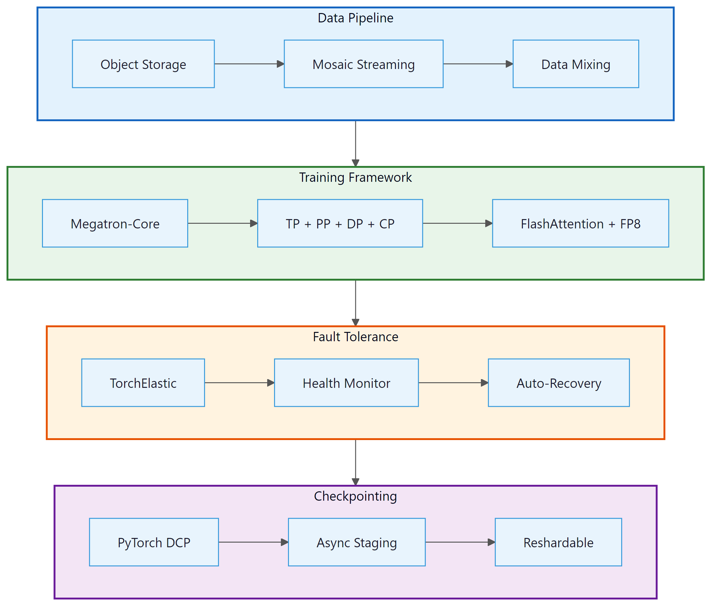
6.8.6 Putting It All Together: Production Training Architecture
A production LLM training system integrates all of the components discussed in this section. The following diagram shows how they fit together for a typical 70B+ model pretraining run:
Several active research directions aim to push training efficiency further. Fully asynchronous pipeline parallelism (e.g., PipeDream-2BW, zero-bubble PP) seeks to eliminate pipeline bubble overhead entirely. Communication-computation overlap research focuses on hiding all-reduce latency behind computation through fine-grained scheduling. FP4 training is an emerging area where 4-bit floating point could double throughput again on next-generation hardware, though maintaining training stability at this precision remains challenging. Heterogeneous training explores using a mix of GPU generations (A100 + H100) in the same cluster, which requires adaptive load balancing to account for different compute speeds.
- Production LLM training requires composing multiple parallelism axes (TP, PP, DP, CP) simultaneously. Megatron-LM/Megatron-Core is the standard framework for this, with configurations tailored to model size and cluster topology.
- MoE models add Expert Parallelism and require load balancing (via auxiliary loss or bias terms) to prevent straggler effects from uneven token routing.
- torch.compile with TorchInductor generates fused Triton kernels that improve training throughput by 10-30%. FlashAttention-2/3 is essential for efficient attention computation, and FP8 training with Transformer Engine nearly doubles H100 throughput.
- Fault tolerance via TorchElastic enables automatic recovery from node failures through elastic re-rendezvous and checkpoint-based restart, essential for multi-week runs on thousands of GPUs.
- PyTorch Distributed Checkpoint (DCP) provides parallel, reshardable, async-capable checkpointing that eliminates the storage bottleneck for large model states.
- Streaming dataset libraries (Mosaic Streaming, WebDataset) provide deterministic, resumable data loading from cloud storage with support for data mixing and curriculum learning.
1. You have 64 GPUs with 80 GB each and a 30B parameter model. Roughly how much memory do the model weights, gradients, and AdamW states require in FP32? Which parallelism strategies (TP, PP, DP, FSDP) would you combine, and why?
Show Answer
2. Explain why pipeline parallelism introduces "bubble" time and how interleaving micro-batches reduces it.
Show Answer
3. A training run on 512 GPUs loses one node every 8 hours on average. Describe how TorchElastic and asynchronous distributed checkpointing keep the run progressing despite these failures.
Show Answer
Exercises
You have a cluster of 256 H100 GPUs (32 nodes with 8 GPUs each) and want to train a 13B parameter model with a 4K context length. Design a parallelism configuration (TP, PP, DP, CP) and justify each choice. What changes if you increase the context to 32K tokens?
Answer Sketch
For 13B at 4K context: TP=2 (model fits in 2 GPUs per layer), PP=1 (small enough for single pipeline stage), DP=128 (256/2/1), CP=1 (short context). For 32K context: increase TP=4 to handle larger activation memory, consider CP=2, giving DP=256/(4*1*2)=32. The key constraint is that TP should stay within a single node for NVLink bandwidth, and CP helps when attention memory becomes the bottleneck at longer sequences.
A 70B model training run has an MTBF of 3,000 iterations. Each iteration takes 30 seconds. A blocking checkpoint takes 5 minutes, and an async checkpoint takes 10 seconds of GPU blocking time. Calculate the optimal checkpoint frequency for both blocking and async cases. How much total GPU-time is saved by using async checkpointing over a 100,000-iteration run?
Answer Sketch
For blocking: optimize $C/6000 + 300/(30 \cdot C)$, giving $C \approx \sqrt{300 \cdot 6000/30} \approx 245$ iterations. For async: $C/6000 + 10/(30 \cdot C)$, giving $C \approx \sqrt{10 \cdot 6000/30} \approx 45$ iterations. Over 100K iterations: blocking checkpoints ~408 times at 5 min each = 34 hours blocking. Async checkpoints ~2,222 times at 10 sec = 6.2 hours. Net saving approximately 28 hours of GPU time across the cluster.
Explain why unbalanced expert routing creates a training bottleneck in MoE models. Derive the auxiliary loss formula and explain how the balancing coefficient $\alpha$ affects the trade-off between load balance and model quality.
Answer Sketch
In MoE, each training step waits for all experts to finish. If expert $i$ receives 3x more tokens than expert $j$, the step time is determined by the slowest (most loaded) expert, wasting compute on the underloaded ones. The auxiliary loss $\alpha \cdot N \sum f_i \cdot p_i$ penalizes routing probability ($p_i$) that concentrates tokens ($f_i$) on few experts. Too high $\alpha$ forces uniform routing but prevents specialization (experts cannot differentiate). Too low $\alpha$ allows imbalance. Typical values of $\alpha = 0.01$ to $0.1$ provide a good compromise.
Write a configuration for a Mosaic StreamingDataset that mixes three data sources: 60% web text, 30% code, and 10% instruction-following data. Include local caching, deterministic shuffling, and resumability support. Explain how the data proportions would change if you were implementing a curriculum that upweights code data in the final 20% of training.
Answer Sketch
Configure three streams with proportions [0.6, 0.3, 0.1], shuffle_seed for determinism, local cache paths on NVMe. For curriculum: at 80% completion, change proportions to [0.4, 0.5, 0.1] to upweight code. Mosaic Streaming supports dynamic proportion changes via the StreamingDataset API. Save dataset.state_dict() before changing proportions to ensure exact resumability.
What's Next?
With a solid understanding of how LLMs are pretrained at scale, including scaling laws, data curation, and distributed training infrastructure, we turn to the models themselves. In Chapter 7: Modern LLM Landscape and Model Internals, we survey the major model families (GPT, Llama, Gemini, Mistral, and more), compare their architectures and training recipes, and explore what makes each one unique.