Rate Limits, Convergence & Benchmarking

The benchmark a model topped last quarter is the benchmark it was trained on this quarter.

Eval, Score-Skeptical AI Agent

Having mapped the frontier vendors in Section 7.2, we now turn to the four topics that most directly govern production model selection: rate limits and capacity, what we can infer about the closed-source architectures without seeing the weights, why frontier capabilities are converging, and how to interpret benchmark numbers in the presence of pervasive contamination.

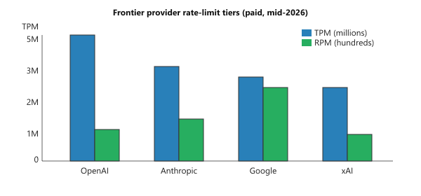
7.2.4 Rate Limits and Practical Constraints

Beyond raw capability and pricing, production deployments must account for rate limits, throughput caps, and availability. Each provider imposes limits on tokens per minute (TPM), requests per minute (RPM), and sometimes requests per day (RPD). These limits vary by pricing tier and can be negotiated for enterprise accounts.

Key practical considerations include:

• Rate limit tiers: Free tier users face strict limits (often 10K-60K TPM). Paid API users get 10x-100x higher limits. Enterprise agreements can remove most caps.
• Batch processing: OpenAI and others offer batch APIs at 50% discounts with 24-hour turnaround, ideal for non-real-time workloads like evaluation, data labeling, or content generation.
• Regional availability: Not all models are available in all regions. European organizations may prefer Mistral or locally hosted alternatives for data residency compliance.
• Model deprecation: Providers regularly deprecate older model versions. Production systems must plan for model migration, which can affect output quality and consistency.

7.2.5 Architectural Insights from the Outside

Although frontier model architectures are proprietary, various signals allow us to infer architectural details:

What We Can Infer

• Mixture of Experts (MoE): GPT-4 is widely believed to use an MoE architecture based on analysis of its behavior and leaked reports. This would explain its strong multi-task performance while keeping inference costs manageable.
• Tokenizer design: API-accessible tokenizers reveal vocabulary size and subword strategies. GPT-4o uses cl100k_base with 100K tokens; Claude uses a custom tokenizer; Gemini's tokenizer handles multimodal inputs natively.
• Context window implementation: The jump from 8K to 128K to 1M contexts suggests different underlying attention mechanisms, likely including some form of sparse attention, sliding window, or hierarchical attention for the longest contexts.
• Post-training pipeline: Anthropic has published details about Constitutional AI. OpenAI has discussed RLHF. Google has described RLAIF (RL from AI Feedback). Each approach produces measurably different model behaviors in terms of safety, helpfulness, and stylistic tendencies.

A Worked Inference: Estimating an MoE's Active Fraction from the Outside

The list above asserts what can be inferred; this subsection turns one of those assertions into a repeatable method, so that "architectural inference" becomes a skill you can apply to any newly released API rather than a claim you take on trust. The target is the most consequential hidden number in a mixture-of-experts model: the ratio of active parameters (the experts actually run per token) to total parameters (the full weight count that must be held in memory). Two observable signals pull in opposite directions and let us bracket it.

The mechanism is this. Autoregressive decode is memory-bandwidth bound: each generated token must read the active weights from GPU memory once, so per-token decode latency scales with active parameters, not total. Price per token, by contrast, must amortize the full served system, including the HBM that holds all experts plus the operator's margin, so price tends to track total capacity. If we have a dense reference model whose active-equals-total parameter count and per-token economics we trust, we can use its latency-per-active-parameter as a yardstick and read the MoE's active count off its measured decode speed. Formally, let $t$ be steady-state decode latency per output token and $P_{\text{act}}$ the active parameter count. Memory-bound decode gives

where $b$ is bytes per parameter (1 for FP8, 2 for BF16), $B_{\text{mem}}$ is the effective memory bandwidth in bytes per second, and the factor 2 counts one multiply-add pair per weight. Bandwidth and precision are hard to know exactly, so rather than solve for $B_{\text{mem}}$ we calibrate it away with a dense reference model of known size: $P_{\text{act}}^{\text{MoE}} \approx P^{\text{ref}} \cdot (t_{\text{MoE}} / t_{\text{ref}})$. The snippet below carries this through with plausible mid-2026 numbers.

# Estimate an MoE model's active-vs-total parameter ratio from the outside,
# using only observable decode latency and price, calibrated against a dense
# reference model whose size we trust. No vendor disclosures required.

# --- Observable signals (illustrative mid-2026 numbers) ---
ref_active_B = 70.0      # dense reference: 70B params, all active
ref_latency_ms = 14.0   # measured per-output-token decode latency
moe_latency_ms = 7.0    # measured decode latency for the MoE under test
moe_price_ratio = 3.0   # MoE output-token price / reference price

# --- Inference 1: active params scale with decode latency (memory-bound) ---
moe_active_B = ref_active_B * (moe_latency_ms / ref_latency_ms)

# --- Inference 2: price tracks total served capacity (HBM + margin) ---
# Treat price ratio as a proxy for total-param ratio vs the reference.
moe_total_B = ref_active_B * moe_price_ratio

active_fraction = moe_active_B / moe_total_B
print(f"Estimated active params:  ~{moe_active_B:.0f}B")
print(f"Estimated total params:   ~{moe_total_B:.0f}B")
print(f"Active fraction:          ~{100*active_fraction:.0f}%")

# --- Error bars: propagate +/-20% uncertainty on each measured ratio ---
lo = (moe_active_B * 0.8) / (moe_total_B * 1.2)
hi = (moe_active_B * 1.2) / (moe_total_B * 0.8)
print(f"Active fraction range:    ~{100*lo:.0f}% to ~{100*hi:.0f}%")

The assumptions are worth naming because they are where the estimate can break. We assume decode is memory-bound (true for single-stream generation, less so for large-batch serving where compute dominates), that the reference model runs on comparable hardware and precision (otherwise $B_{\text{mem}}$ does not cancel cleanly), and that price reflects cost rather than strategic discounting (a vendor subsidizing a launch breaks Inference 2). The +/-20 percent error bars on each measured ratio compound into a roughly 11 to 25 percent active-fraction band, wide enough that you should treat the point estimate as an order-of-magnitude read, not a spec sheet. The skill transfers: the same calibrate-against-a-known-reference move lets you infer KV-cache footprint from context-length pricing breaks, or quantization level from a latency drop that is too large to be a model change. Architectural inference is not guesswork; it is dimensional analysis against signals the provider cannot hide.

# Inspecting tokenizer behavior across providers
import tiktoken
# OpenAI GPT-4o tokenizer
enc = tiktoken.encoding_for_model("gpt-4o")
text = "The quick brown fox jumps over the lazy dog."
tokens = enc.encode(text)
print(f"GPT-4o tokens: {len(tokens)}")
print(f"Token IDs: {tokens}")
print(f"Decoded tokens: {[enc.decode([t]) for t in tokens]}")
# Compare: How different models tokenize the same multilingual text
multilingual = "Hello world. Bonjour le monde. Hola mundo."
print(f"\nMultilingual text tokens: {len(enc.encode(multilingual))}")
# Different tokenizers will produce different token counts,
# reflecting their training data distribution

7.2.6 The Convergence Trend

A striking trend in the frontier model landscape is convergence. In 2023, GPT-4 held a commanding lead on most benchmarks. By 2025, Claude, Gemini, and even some open-weight models have closed much of the gap. On many practical tasks, the differences between frontier models are smaller than the differences caused by prompt engineering choices or task-specific fine-tuning.

This convergence has several implications for practitioners:

1. Multi-provider strategies reduce risk: If your application's prompts work well across Claude, GPT-4o, and Gemini, you gain resilience against outages, pricing changes, and deprecation.
2. Differentiation moves to the edges: The competitive advantage increasingly comes from context length, multimodal capabilities, tool use, latency, or specialized enterprise features rather than raw text generation quality.
3. Open models are catching up: As we will see in Section 7.3, open-weight models now approach frontier capability on many tasks, raising questions about the long-term value proposition of closed-source alternatives.

7.2.7 Benchmarking Methodology and Contamination

As frontier models converge in capability, the methodology used to compare them has become as important as the models themselves. A difference of 2 to 3 percentage points on a benchmark may reflect genuine capability gaps, prompt engineering differences, evaluation contamination, or simply statistical noise. Practitioners must understand how benchmarks work and where they break down to make informed model selection decisions.

Chatbot Arena: Human Preference at Scale

The LMSYS Chatbot Arena, launched by UC Berkeley researchers in 2023, has become the most trusted model comparison platform. Its methodology is simple: users submit a prompt, receive responses from two anonymous models side by side, and vote for the better response. The platform then computes Elo ratings (borrowed from chess) to produce a global ranking. By early 2025, Chatbot Arena has collected over 1 million human preference votes across hundreds of models. Several properties make it uniquely valuable. First, the prompts are user-generated and diverse, covering everything from creative writing to technical debugging, rather than drawn from a fixed test set that models might have seen during training. Second, the blind evaluation eliminates brand bias. Third, the Elo system naturally accounts for the relative difficulty of comparisons.

However, Chatbot Arena has limitations. Its user base skews toward English-speaking technical users, so the rankings may not reflect performance on non-English tasks or non-technical domains. Votes are influenced by presentation factors (formatting, length, tone) that may not correlate with accuracy. The platform has introduced category-specific leaderboards (coding, math, reasoning, hard prompts) to provide more granular signal, and "Arena Hard Auto," a static benchmark of 500 challenging prompts evaluated by GPT-4o as a judge, provides a reproducible approximation of the full Arena experience.

Benchmark Contamination

Contamination occurs when a model has seen benchmark questions or answers during training, inflating its scores beyond its true capability. As training datasets have grown to trillions of tokens scraped from the open web, contamination has become a systemic concern. MMLU questions appear on study websites. HumanEval coding problems circulate on forums. GSM8K math problems are reproduced in educational content. The result is that a model's score on a contaminated benchmark reflects a mixture of genuine reasoning ability and memorized answers, and it is difficult to separate the two.

Several approaches have emerged to address contamination. Dynamic benchmarks like LiveCodeBench (which draws new coding problems from competitive programming contests published after a cutoff date) and GAIA (which tests general AI assistants on novel, manually crafted tasks) resist contamination by being continuously updated. Canary string detection involves embedding unique identifiers in benchmark data and then checking whether models can reproduce them, indicating memorization. Holdout evaluation sets are maintained privately by evaluation organizations and never published, though this limits reproducibility. The BigCodeBench and LiveBench projects combine dynamic generation with automated verification to provide contamination-resistant evaluation at scale.

Best Practices for Model Evaluation

Given these challenges, practitioners should adopt a multi-layered evaluation strategy. Start with Chatbot Arena rankings and Arena Hard Auto for a general capability signal. Use domain-specific benchmarks relevant to your use case (for example, MedQA for healthcare, FinBench for finance, or SWE-bench for software engineering). Build a private evaluation set of 100 to 500 examples drawn from your actual production distribution, annotated by domain experts. Run this evaluation whenever you consider switching models or upgrading to a new version. Track not just accuracy but also consistency (does the model give the same answer to the same question across multiple runs?), latency, and cost. No single benchmark captures everything that matters for a production application; the combination of public benchmarks, domain benchmarks, and private evaluation provides the most reliable signal.