The Test-Time Compute Paradigm

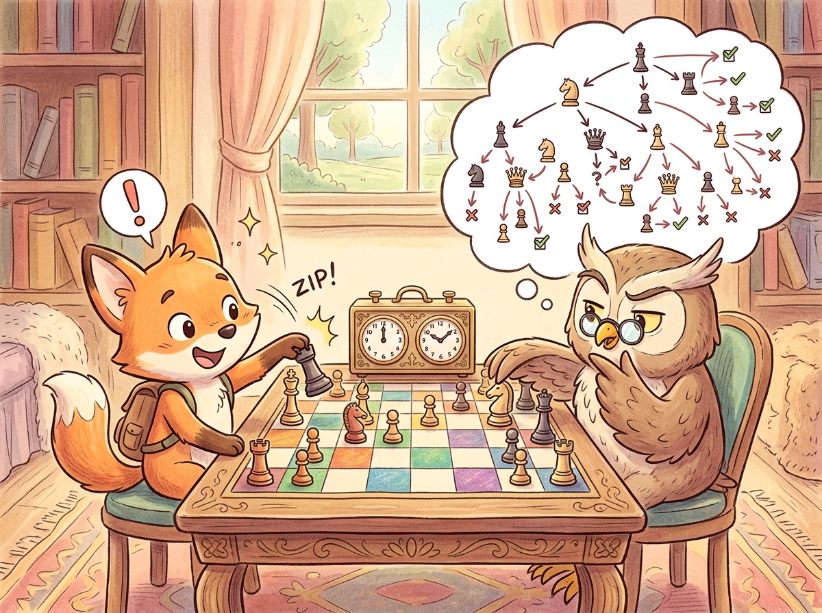
A wise person does not give the same amount of thought to choosing lunch as to choosing a career. Neither should a language model.

Chinchilla, Wisely Allocating AI Agent

1. Two Kinds of Compute

Every language model consumes compute in two distinct phases. Understanding the distinction is essential for grasping why reasoning models represent a paradigm shift.

Train-time compute is the total processing power consumed during pre-training and post-training. This includes the GPU hours spent on next-token prediction over trillions of tokens, followed by supervised fine-tuning and alignment (see Chapter 17). Train-time compute is a one-time investment: once the model weights are set, the cost is amortized across every future inference request. Larger models with more parameters require proportionally more training compute, but serve every user with the same fixed set of weights.

Test-time compute (also called inference-time compute) is the processing power consumed each time the model generates a response. In a standard LLM, this cost is approximately proportional to the number of output tokens: each token requires one forward pass through the network. In a reasoning model, the cost per query can vary enormously. A simple factual question might consume 50 tokens of thinking, while a hard mathematical proof might consume 10,000 or more.

1.1 The Classical Scaling Regime

The Kaplan scaling laws (2020) established that language model loss decreases as a power law in three variables: number of parameters $N$, dataset size $D$, and total training compute $C$. The Chinchilla correction (Hoffmann et al., 2022) refined this by showing that models should scale parameters and data equally: a model with $N$ parameters should be trained on approximately $20N$ tokens for compute-optimal training.

These laws predict diminishing returns: doubling training compute yields a roughly 10% reduction in loss. To cut loss in half, you need to increase compute by roughly 100x. At the frontier, where training runs already cost $100M+, this creates severe economic pressure. (For the full derivation and historical context, see Section 06.3.)

1.2 The Test-Time Scaling Regime

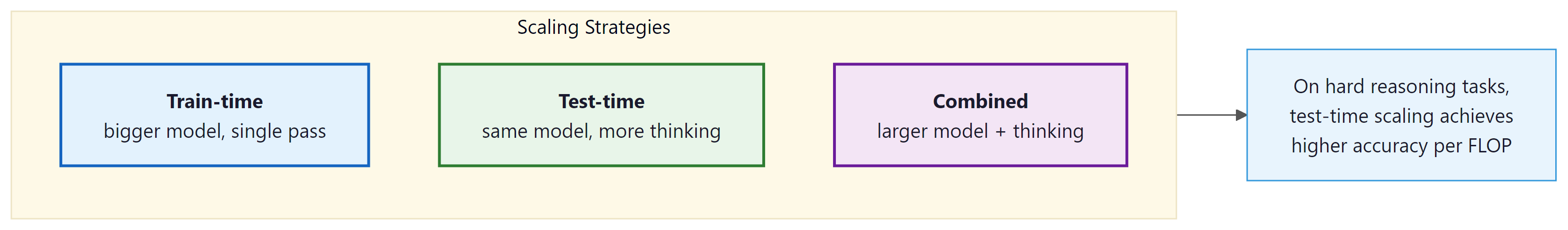
Test-time compute scaling offers a fundamentally different trade-off. Instead of spending more at training to improve the model for all queries equally, you spend more at inference to improve the model's response to a specific query. This has several important properties:

• Per-query cost: Unlike training, which is amortized, test-time compute is a direct per-query cost. A reasoning model that generates 5,000 thinking tokens costs roughly 50x more than a standard model generating 100 tokens.
• Adaptive allocation: The compute can be allocated proportional to difficulty. Easy queries receive minimal thinking; hard queries receive extensive deliberation. This means the average cost per query can be much lower than the worst case.
• Complementary to train-time scaling: A model can be both well-trained and equipped with test-time reasoning. The two forms of scaling are additive, not substitutes. A reasoning model trained with more compute will reason better than a smaller one.
• Immediate deployment: Improving test-time scaling does not require retraining the model. Techniques like best-of-N sampling or tree search can be applied to any model at serving time (though purpose-trained reasoning models perform best).

Figure 8.1.2: Performance as a function of total compute under three scaling strategies. On hard reasoning tasks, test-time scaling (green) achieves higher accuracy per FLOP than simply using a larger model (purple). The combined approach (red dashed) pushes the frontier further.

2. The Snell et al. Framework

The foundational paper for understanding test-time compute is Snell et al. (2024), "Scaling LLM Test-Time Compute Optimally can be More Effective than Scaling Model Parameters." This work provides the theoretical and empirical framework for answering a simple question: given a fixed compute budget for a single inference query, how should you allocate that budget between model size and test-time reasoning?

2.1 The Compute-Optimal Inference Problem

Consider a scenario where you have a fixed inference compute budget $C$ FLOPs per query. You can spend this budget in several ways:

1. Single pass through a large model: Use all $C$ FLOPs for one forward pass through the largest model that fits within the budget. This is the classical approach.
2. Multiple passes through a smaller model: Use a model that requires $C/N$ FLOPs per pass and generate $N$ independent solutions, then select the best one using a reward model.
3. Extended chain-of-thought with a medium model: Use a model that generates a long reasoning trace, spending extra tokens to "think through" the problem before committing to an answer.
4. Tree search with a small model: Use a small model to explore a tree of partial solutions, using a reward model to guide the search toward promising branches.

Snell et al. show that the optimal strategy depends critically on task difficulty. Their key finding can be summarized in one sentence: on hard problems where a base model achieves less than 50% accuracy, test-time compute scaling with a smaller model can match or exceed a 14x larger model using the same total FLOPs.

2.2 Difficulty-Dependent Optimality

3. Mechanisms of Test-Time Compute

There are three primary mechanisms through which a model can invest additional compute at inference time. Each represents a different approach to the same goal: generating better answers by spending more processing per query.

3.1 Extended Chain-of-Thought

The most visible mechanism in modern reasoning models is extended chain-of-thought (CoT). The model generates a long sequence of "thinking tokens" before producing its final answer. These tokens represent the model's internal deliberation: breaking the problem into steps, considering alternatives, checking intermediate results, and sometimes backtracking when it detects an error.

In OpenAI's o1 and o3, these thinking tokens are hidden from the user (the API returns only a summary). In DeepSeek R1, the thinking process is visible, enclosed in <think>...</think> tags. The number of thinking tokens varies adaptively: a simple arithmetic question might generate 50 thinking tokens, while a competition-level math problem might generate 10,000+.

Why thinking tokens help, mechanically. A transformer is a fixed-depth computation graph: each input token passes through the same number of layers regardless of problem difficulty. By generating intermediate reasoning tokens, the model effectively gives itself additional "layers" of processing. Each thinking token feeds back into the context, allowing subsequent computations to build on earlier ones. This converts a fixed-depth computation into an adaptive-depth one, which is necessary for problems that require compositional reasoning (multi-step math, logical deduction, code debugging). The cost is linear in the number of thinking tokens, but the problems it unlocks are qualitatively different from what a single forward pass can solve. For deployment, this means the KV cache grows proportionally with thinking tokens, making efficient memory management crucial.

# Comparing standard vs. reasoning model outputs on the same problem
# Problem: "What is the sum of all prime numbers less than 20?"

# === Standard Model (GPT-4o) ===
# Output: "The prime numbers less than 20 are: 2, 3, 5, 7, 11, 13, 17, 19.
# Their sum is 2 + 3 + 5 + 7 + 11 + 13 + 17 + 19 = 77."
# Tokens generated: ~40
# Time: ~0.5s

# === Reasoning Model (o3-mini) ===
# Hidden thinking tokens (~200 tokens):
# "I need to find all primes less than 20.
# Starting from 2: 2 is prime.
# 3 is prime (not divisible by 2).
# 4 = 2x2, not prime.
# 5 is prime (not divisible by 2 or 3).
# 6 = 2x3, not prime.
# 7 is prime (not divisible by 2, 3, or 5). Actually I only need
# to check up to sqrt(7) ~ 2.6, so just check 2. Not divisible. Prime.
# ...
# [continues for all numbers up to 19]
# Now summing: 2+3=5, 5+5=10, 10+7=17, 17+11=28, 28+13=41,
# 41+17=58, 58+19=77.
# Let me verify: 2,3,5,7,11,13,17,19. Count: 8 primes. Sum: 77."
# Visible output: "The sum of all prime numbers less than 20 is 77."
# Total tokens (thinking + output): ~250
# Time: ~2s

# The reasoning model consumed ~6x more tokens but used a more
# systematic verification process. For this easy problem, both
# get the right answer. The difference becomes dramatic on harder
# problems where the standard model would make errors.

3.2 Best-of-N Sampling

A conceptually simpler approach is to generate $N$ independent solutions and select the best one. This requires a reward model (or verifier) that can score each candidate solution. The approach is "embarrassingly parallel" since all N candidates can be generated simultaneously on separate GPUs.

Performance scales logarithmically with $N$: doubling the number of samples yields a roughly constant improvement in accuracy. This means that going from N=1 to N=8 provides a large boost, but going from N=64 to N=128 provides a much smaller one. Practical systems typically use N between 8 and 64, balancing cost against accuracy.

3.3 Tree Search

Tree search methods, including Monte Carlo Tree Search (MCTS) and beam search variants, structure the reasoning process as an explicit search over partial solutions. Each node in the tree represents a partial chain of thought, and edges represent possible next reasoning steps. A reward model evaluates the promise of each partial solution, allowing the search to focus compute on the most promising reasoning paths.

Tree search is more compute-efficient than best-of-N for hard problems because it avoids wasting compute on completely wrong solution paths. If the first reasoning step is clearly wrong, tree search can detect this early (via the reward model) and redirect compute to better branches. Best-of-N, by contrast, generates each solution independently and can repeat the same mistakes across many of its N attempts.

We cover tree search in detail in Section 8.5, including AlphaProof's application of MCTS to formal mathematical reasoning.

3.4 Reasoning Architecture Taxonomy

The term "reasoning model" covers at least four meaningfully different architectural choices. They share the goal of allocating more compute to harder problems, but differ in where the reasoning lives, who can see it, and how it is structured. Understanding these distinctions matters for choosing the right model in production and for interpreting benchmark comparisons.

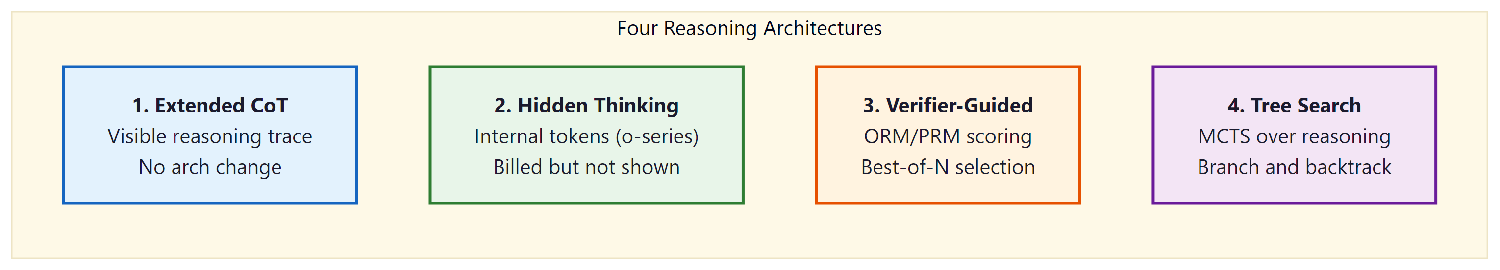
Figure 8.1.3: The four major reasoning architecture approaches compared. Extended CoT adds no new architecture but trains the model to reason longer. Hidden thinking (o-series) uses RL to produce internal reasoning tokens invisible to the user. Explicit thinking (DeepSeek R1) exposes the reasoning trace via <think> tags. Tree search (MCTS) generates and scores multiple reasoning branches, requiring a process reward model.

Extended Chain-of-Thought is the simplest approach architecturally: the model is the same transformer, but it is trained (or prompted) to produce long reasoning traces before the answer. No structural change to the model is required. The reasoning trace is visible in the output and can be inspected, which makes it useful for debugging. The limitation is that quality depends heavily on training, and a model trained only with prompting (rather than RL) may not learn when to stop reasoning.

Hidden Thinking is the approach used by OpenAI's o-series (o1, o3, o4-mini). The model is trained with reinforcement learning to produce internal reasoning tokens that are not returned in the API response. The thinking tokens are generated autoregressively and consume full KV cache memory during generation, but are stripped before the response is returned. From the user's perspective, the model appears to pause and then return a concise answer. The tradeoff is interpretability: you cannot inspect the reasoning, which makes debugging failures harder. (See Section 8.2 for the o-series architecture in detail.)

Explicit Thinking is the approach used by DeepSeek R1. The model outputs its reasoning trace enclosed in <think>...</think> XML tags, followed by the final answer. The trace is part of the response and can be read, cached, and used for fine-tuning or distillation. DeepSeek-AI (2025) showed that this behavior can emerge from pure reinforcement learning, without supervised chain-of-thought data, using their GRPO training algorithm. Because the trace is visible, it is significantly easier to debug why the model failed on a given problem. The tradeoff is that the full trace appears in the response, which increases output token count and therefore cost.

Tree Search (MCTS-style) represents a fundamentally different approach. Instead of generating one linear reasoning trace, the model generates multiple reasoning branches, scores each with a reward model, and expands the most promising ones. This is similar to Monte Carlo Tree Search as used in game-playing AI (AlphaGo, AlphaProof). The compute cost is substantially higher than linear CoT because multiple partial solutions are generated and evaluated. However, for problems that require finding a specific correct reasoning path among many plausible-looking wrong paths (olympiad mathematics, formal proofs, complex constraint satisfaction), tree search can find solutions that linear CoT misses entirely. A process reward model (Section 7) is essential for tree search to work: you need step-level scoring to prune bad branches early.

3.5 Best-of-N Sampling: Depth vs. Breadth

Best-of-N (also called rejection sampling) occupies the middle ground between simple extended CoT and expensive tree search. Generate $N$ complete independent reasoning chains from the same model, score each with a reward model, and return the highest-scoring response. The approach is "embarrassingly parallel" since all N chains can be generated simultaneously.

Compute cost is linear in N, but quality improvement is logarithmic. If the probability of any single chain being correct is $p$, then the probability of at least one correct solution among N samples is $1 - (1-p)^N$. This grows quickly at first (N=1 to N=8 gives a large boost) and then saturates (N=64 to N=128 gives a small boost). In practice, N between 8 and 64 covers most of the achievable gain.

import anthropic
import math

def best_of_n(prompt: str, n: int, score_fn) -> str:
 """
 Generate N independent responses and return the highest-scoring one.

 score_fn: callable that takes a response string and returns a float score.
 This could be a rule-based verifier (e.g., check if math answer is numeric
 and matches ground truth format) or a separate reward model API call.
 """
 client = anthropic.Anthropic()

 # Generate N independent responses (in practice, batch these in parallel)
 responses = []
 for _ in range(n):
 msg = client.messages.create(
 model="claude-opus-4-5",
 max_tokens=1024,
 messages=[{"role": "user", "content": prompt}]
 )
 responses.append(msg.content[0].text)

 # Score each response and pick the best
 scored = [(score_fn(r), r) for r in responses]
 best_score, best_response = max(scored, key=lambda x: x[0])

 return best_response

# Example: verifiable math problem
def math_verifier(response: str) -> float:
 """Simple rule-based verifier: does the response contain a numeric answer?"""
 import re
 # Look for a final answer pattern like "= 42" or "answer is 42"
 matches = re.findall(r'(?:=|answer is|result is)\s*([\d,\.]+)', response.lower())
 return 1.0 if matches else 0.0

# Expected accuracy improvement with best-of-N
# If single-sample accuracy = 30%, best-of-N accuracy (theoretical ceiling):
p = 0.30
for n in [1, 4, 8, 16, 32, 64]:
 ceiling = 1 - (1 - p) ** n
 print(f"N={n:3d}: theoretical ceiling = {ceiling:.1%}")

Relationship to rejection sampling in RLHF training. The same best-of-N principle underlies a key step in RLHF: during the supervised fine-tuning warm-up, the model generates multiple responses to each prompt, and the best response (as scored by a reward model) is used as the training target. This is called rejection sampling fine-tuning (RFT) and is how DeepSeek-R1 created its supervised warm-up data. For full RLHF context, see Section 17.1.

When to prefer best-of-N over tree search. Best-of-N is simpler to implement (no partial-solution infrastructure), works with any model without modification, and has predictable cost (exactly N forward passes). Tree search has higher overhead (partial solutions must be tracked, the tree must be maintained, and a PRM is required) but is more compute-efficient on very hard problems. A practical rule: start with best-of-N at N=8 to 32; only move to tree search if best-of-N is still failing.

These reasoning strategies are powerful, but they are not free. Every additional thinking token costs compute, latency, and memory. Before deploying any of these approaches, you need to understand the cost structure and learn how to budget reasoning compute effectively.

4. The Economics of Thinking

Test-time compute introduces a new dimension to the economics of LLM inference. The cost per query is no longer approximately fixed; it varies with problem difficulty and the chosen reasoning budget.

4.1 Token Costs

Reasoning models typically charge for both thinking tokens and output tokens, though the pricing structure varies. As of early 2025:

A critical detail: reasoning models generate far more tokens per query than standard models. A query that costs $0.001 with GPT-4o (100 output tokens) might cost $0.05 to $0.20 with o3 (1,000 to 5,000 thinking + output tokens). The per-token price of reasoning models is sometimes lower, but the total cost per query is typically 5x to 50x higher because of the additional thinking tokens.

4.2 The Routing Optimization

The wide variance in per-query cost creates a strong incentive for intelligent routing: sending easy questions to cheap, fast models and reserving expensive reasoning models for hard questions. This is not merely a cost optimization; it also improves latency. A simple factual query answered by GPT-4o-mini in 200ms is a better user experience than the same query sent to o3, which might take 5 to 15 seconds as it "thinks" about something that needs no thought.

Effective routing requires a difficulty estimator. This can be as simple as a logistic regression classifier trained on labeled query difficulty, or as sophisticated as a small language model fine-tuned to predict whether a reasoning model would produce a better answer than a standard model. The difficulty estimator itself is cheap to run (typically a single forward pass through a small model) and acts as a gatekeeper that protects the reasoning model from wasting compute on trivial queries.

5. Historical Context: From Chain-of-Thought to Reasoning Models

The reasoning model paradigm did not emerge in a vacuum. It builds on a decade of research into improving language model reasoning, with each advance building on the last.

1. 2017: Scratchpad method. Nye et al. showed that letting models write intermediate computation steps (a "scratchpad") improved performance on algorithmic tasks. This was the first evidence that visible intermediate reasoning helps.
2. 2022: Chain-of-thought prompting. Wei et al. demonstrated that simply prompting a model to "think step by step" dramatically improved reasoning accuracy. This required no model changes, just a prompt modification.
3. 2022: Self-consistency. Wang et al. showed that sampling multiple chain-of-thought solutions and taking a majority vote improved accuracy beyond a single CoT sample. This introduced the idea that more inference-time samples yield better answers.
4. 2022: STaR. Zelikman et al. proposed Self-Taught Reasoner, which iteratively fine-tunes a model on its own correct reasoning traces. This bootstrapping approach was an early precursor to training models specifically for reasoning.
5. 2023: Process reward models. Lightman et al. (PRM800K) demonstrated that rewarding individual reasoning steps outperforms rewarding only final answers, laying the groundwork for step-level supervision in reasoning models.
6. 2024: OpenAI o1. The first commercially deployed reasoning model, trained with reinforcement learning to produce extended chains of thought. Hidden reasoning tokens, RL-trained rather than prompt-elicited.
7. 2025: DeepSeek R1. Open-weight reasoning model demonstrating that reasoning behavior emerges from pure RL (R1-Zero) without supervised CoT data. Introduced GRPO training and <think> token delimiters.
8. 2025: Reasoning proliferation. Google Gemini 2.5 (thinking mode), Qwen QwQ, Kimi k1.5, o3, o4-mini. Reasoning capabilities become a standard feature rather than a niche capability.

6. When to Use Test-Time Compute

Not every task benefits from reasoning models. The following decision framework helps practitioners identify where test-time compute provides genuine value versus where it is wasted spend.

Use reasoning models when:

• The task requires multi-step logical reasoning (mathematical proofs, code debugging, legal analysis)
• The problem has a verifiable answer (math, code execution, constraint satisfaction)
• Accuracy is more important than latency (batch processing, offline analysis)
• The base model achieves 20% to 80% accuracy (the "sweet spot" for test-time scaling)
• Errors are expensive (medical reasoning, financial analysis, safety-critical systems)

Use standard models when:

• The task is primarily retrieval or summarization (factual lookups, document summarization)
• Latency matters more than marginal accuracy (real-time chat, autocomplete)
• The base model already achieves >90% accuracy (no room for improvement via thinking)
• The task is creative or subjective (writing, brainstorming) where there is no single "right" answer
• Cost per query is tightly constrained

7. KV Cache Growth in Reasoning Models

One of the most consequential engineering challenges with reasoning models is memory. Every token the model generates, including every thinking token, must be stored in the KV cache during the generation pass. For standard chat models generating 200 to 500 tokens, this is manageable. For reasoning models generating 5,000 to 50,000 thinking tokens, it becomes a serious infrastructure problem. (For the technical mechanics of KV cache and its relationship to inference optimization, see Section 9.2.)

7.1 The Memory Arithmetic

The KV cache stores key and value tensors for every token in the context. For a transformer with $L$ layers, $H$ key-value heads, and head dimension $d_h$, the KV cache memory per token is:

$$\text{Memory per token} = 2 \times L \times H \times d_h \times \text{bytes per element}$$

The factor of 2 accounts for both keys and values. For a model using Grouped Query Attention (GQA), the number of KV heads is smaller than the number of query heads, which reduces this cost proportionally.

7.2 Serving Implications

These numbers have direct consequences for how reasoning model deployments are architected:

• Throughput collapse: A GPU that serves 200 concurrent standard chat requests can serve as few as 2 to 5 concurrent reasoning requests at maximum thinking depth. This means the effective cost per reasoning request is not just the token count difference but also the opportunity cost of blocked GPU capacity.
• Prefill/decode phase imbalance: In standard inference, the prefill phase (processing the input prompt) is fast, and the decode phase (generating output tokens one by one) is the bottleneck. In reasoning models, the decode phase is enormously extended by thinking tokens, making decode the dominant cost by far.
• Memory-bound vs. compute-bound: With tens of thousands of tokens in the KV cache, attention computation becomes memory-bandwidth-bound. The GPU spends most of its time reading KV cache tensors from HBM rather than performing matrix multiplications. Flash Attention and GQA (see Section 9.2) are therefore especially valuable for reasoning models.

7.3 Mitigation Strategies

Production deployments use several strategies to manage KV cache growth in reasoning models:

• KV cache eviction after reasoning completes: Once the model emits the separator token (transitioning from thinking to answer), the thinking tokens are no longer needed for future generation. Their KV cache entries can be freed, recovering GPU memory before serving the next request. This is not possible during generation, but can happen between requests.
• Thinking token compression: Research systems have explored compressing or summarizing the KV cache of thinking tokens into a smaller representation. This is an active research area and not yet widely deployed.
• Budget caps: Most reasoning model APIs expose a "reasoning budget" or "thinking effort" parameter. Setting thinking_tokens=1024 caps the maximum KV cache growth and prevents runaway costs on simple queries. OpenAI's o-series exposes reasoning_effort (low, medium, high); DeepSeek R1 supports explicit max_tokens caps on the thinking section. Always set a budget cap for production deployments.
• Routing: The most effective mitigation is simply not sending easy queries to reasoning models. A difficulty router (see Section 4.2) prevents most requests from incurring thinking token overhead at all.

import anthropic

client = anthropic.Anthropic()

# Using Claude's extended thinking with a budget cap to limit KV cache growth.
# budget_tokens limits the maximum thinking tokens, directly capping memory usage.
response = client.messages.create(
 model="claude-opus-4-5",
 max_tokens=16000,
 thinking={
 "type": "enabled",
 "budget_tokens": 2048 # cap thinking tokens: reduces memory from ~640 MB to ~26 MB
 # for a 70B-equivalent model. Default can be up to 10000.
 },
 messages=[{
 "role": "user",
 "content": "Prove that the square root of 2 is irrational."
 }]
)

# Response includes both thinking blocks and text blocks
for block in response.content:
 if block.type == "thinking":
 print(f"Thinking ({len(block.thinking)} chars): {block.thinking[:200]}...")
 elif block.type == "text":
 print(f"Answer: {block.text}")

8. Process Reward Models vs. Outcome Reward Models

Every reasoning strategy that involves evaluation (best-of-N, tree search, and RL training of reasoning models) requires a reward model. Not all reward models are created equal. The choice between an outcome reward model (ORM) and a process reward model (PRM) fundamentally affects what can be achieved.

8.1 Outcome Reward Models

An ORM scores the final answer only. Given a problem and a complete reasoning trace plus final answer, the ORM outputs a single scalar: how good is this answer? ORMs are relatively easy to train because labels are at the answer level: for math problems, you can automatically verify whether the final numerical answer is correct. For code, you can run tests. The feedback is binary and abundant.

The limitation of ORMs is sparse signal. If a 50-step reasoning chain arrives at the wrong answer, the ORM assigns a low score to the entire chain, but provides no information about which of the 50 steps went wrong. This makes ORMs poorly suited for tree search (you cannot prune a bad branch until you reach the end of it) and for training (the gradient signal does not flow back to the specific reasoning step that caused the error).

8.2 Process Reward Models

A PRM scores each individual reasoning step. Given a problem and the reasoning trace up to step $k$, the PRM outputs a score for whether step $k$ was correct and productive. This provides dense, step-level supervision: the model receives a signal at every step, not just at the end.

The foundational work is Lightman et al. (2023), "Let's Verify Step by Step," which introduced the PRM800K dataset: 800,000 step-level human annotations on math reasoning traces. Their key finding was that PRMs substantially outperform ORMs on hard math benchmarks, particularly when used for best-of-N selection. Given N candidate solutions, a PRM can score each step of each solution and select the one with the highest minimum step score (the weakest link), which is a more reliable quality signal than the final-answer score alone.

8.3 Automated PRM Training

The cost of step-level human annotation has motivated research into automated PRM training. Two approaches have shown promise:

• Monte Carlo rollout estimation: For a given partial reasoning trace ending at step $k$, generate many complete solutions (rollouts) from step $k$ forward. The fraction of rollouts that arrive at the correct final answer estimates the probability that step $k$ is on a path to success. This probability is used as the step-level label. The DeepSeek-R1 team used this technique to generate PRM training data at scale.
• LLM-as-critic: Use a separate language model to evaluate whether each reasoning step is logically valid. This is cheaper than human annotation but introduces the risk of the critic having the same biases as the generator. Best practice is to use a different model family for the critic than for the generator.

For the RL training context (how PRMs and ORMs connect to PPO, GRPO, and DPO during reasoning model training), see Section 17.1.

Exercises