The KV cache wanted to grow. It wanted to grow at every token, on every layer, in every head. I told it about quantization. It grew anyway, just more slowly.
KV, Cache-Aware AI Agent
This section continues from Section 8.1, which introduced the two kinds of compute, the Snell et al. framework, the four mechanisms of test-time compute, the economics of thinking, the historical path from chain-of-thought to reasoning models, and when to use test-time compute. Here we turn to the two engineering realities that matter most when you actually deploy a reasoning model: KV cache growth under long thinking traces, and the choice between Process and Outcome Reward Models for scoring those traces. The section closes with exercises that consolidate the full test-time-compute picture.
Prerequisites
This section continues from Section 8.1. Familiarity with the four mechanisms of test-time compute (extended CoT, hidden thinking, explicit thinking, tree search), the Snell et al. compute-optimality framework, and the basic chain-of-thought paradigm covered there is assumed.
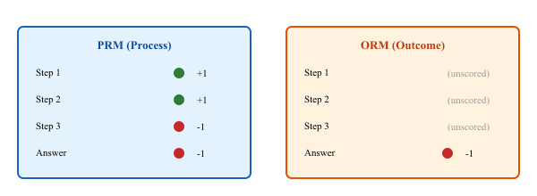
Outcome Reward Models scored only the final answer, so they often gave full credit to lucky guesses and zero credit to a near-miss with perfect intermediate work. Process Reward Models, by scoring each step, turned what looked like 'this kid is bad at math' into 'this kid forgot to carry the one'. The pedagogy was already known to every grade-school teacher in the world. The interesting thing is that it took a few billion parameters of reasoning research to rediscover it.
Having framed why test-time compute matters in Section 8.1, we now look at the two engineering realities that govern production deployment: how the KV cache explodes under long reasoning traces, and how PRMs and ORMs differ in how they score those traces.
8.1.7 KV cache Growth in Reasoning Models
One of the most consequential engineering challenges with reasoning models is memory. Every token the model generates, including every thinking token, must be stored in the KV cache during the generation pass. For standard chat models generating 200 to 500 tokens, this is manageable. For reasoning models generating 5,000 to 50,000 thinking tokens, it becomes a serious infrastructure problem. (For the technical mechanics of KV cache and its relationship to inference optimization, see Section 9.3.)
8.1.7.1 The Memory Arithmetic
The KV cache stores key and value tensors for every token in the context. For a transformer with $L$ layers, $H$ key-value heads, and head dimension $d_h$, the KV cache memory per token is:
The factor of 2 accounts for both keys and values. For a model using Grouped Query Attention (GQA), the number of KV heads is smaller than the number of query heads, which reduces this cost proportionally.
Consider a 70B parameter model using GQA with the following typical configuration:
- Layers: 80
- KV heads (GQA): 8 (query heads: 64)
- Head dimension: 128
- Precision: fp16 (2 bytes per element)
KV cache per token: 2 (K+V) x 80 (layers) x 8 (KV heads) x 128 (head dim) x 2 (bytes) = 327,680 bytes per token, or about 320 KB per token.
For 50,000 thinking tokens: 50,000 x 320 KB = 16 GB of KV cache, for a single request. A standard 80 GB A100 can serve roughly 5 concurrent requests of this depth. For comparison, a standard 500-token chat response uses only 160 MB of KV cache (100x less).
If the GQA ratio is larger (e.g., 4 KV heads instead of 8), the memory roughly halves, but the order of magnitude remains the same: long reasoning traces consume gigabytes of GPU memory per request.
8.1.7.2 Serving Implications
These numbers have direct consequences for how reasoning model deployments are architected:
- Throughput collapse: A GPU that serves 200 concurrent standard chat requests can serve as few as 2 to 5 concurrent reasoning requests at maximum thinking depth. This means the effective cost per reasoning request is not just the token count difference but also the opportunity cost of blocked GPU capacity.
- Prefill/decode phase imbalance: In standard inference, the prefill phase (processing the input prompt) is fast, and the decode phase (generating output tokens one by one) is the bottleneck. In reasoning models, the decode phase is enormously extended by thinking tokens, making decode the dominant cost by far.
- Memory-bound vs. compute-bound: With tens of thousands of tokens in the KV cache, attention computation becomes memory-bandwidth-bound. The GPU spends most of its time reading KV cache tensors from HBM rather than performing matrix multiplications. FlashAttention and GQA (see Section 9.3) are therefore especially valuable for reasoning models.
8.1.7.3 Mitigation Strategies
Production deployments use several strategies to manage KV cache growth in reasoning models:
- KV cache eviction after reasoning completes: Once the model emits the separator token (transitioning from thinking to answer), the thinking tokens are no longer needed for future generation. Their KV cache entries can be freed, recovering GPU memory before serving the next request. This is not possible during generation, but can happen between requests.
- Thinking token compression: Research systems have explored compressing or summarizing the KV cache of thinking tokens into a smaller representation. This is an active research area and not yet widely deployed.
- Budget caps: Most reasoning model APIs expose a "reasoning budget" or "thinking effort" parameter. Setting
thinking_tokens=1024caps the maximum KV cache growth and prevents runaway costs on simple queries. OpenAI's o-series exposesreasoning_effort(low, medium, high); DeepSeek R1 supports explicitmax_tokenscaps on the thinking section. Always set a budget cap for production deployments. - Routing: The most effective mitigation is simply not sending easy queries to reasoning models. A difficulty router (see Section 4.2) prevents most requests from incurring thinking token overhead at all.
import anthropic
client = anthropic.Anthropic()
# Using Claude's extended thinking with a budget cap to limit KV cache growth.
# budget_tokens limits the maximum thinking tokens, directly capping memory usage.
response = client.messages.create(
    model="claude-opus-4-5",
    max_tokens=16000,
    thinking={
    "type": "enabled",
    "budget_tokens": 2048 # cap thinking tokens: reduces memory from ~640 MB to ~26 MB
    # for a 70B-equivalent model. Default can be up to 10000.
    },
    messages=[{
    "role": "user",
    "content": "Prove that the square root of 2 is irrational."
    }]
    )
# Response includes both thinking blocks and text blocks
for block in response.content:
    if block.type == "thinking":
        print(f"Thinking ({len(block.thinking)} chars): {block.thinking[:200]}...")
    elif block.type == "text":
print(f"Answer: {block.text}")budget_tokens cap on extended thinking using the Anthropic Python SDK. The cap directly limits KV cache memory growth. For a 70B-equivalent model, cutting thinking from 10,000 to 2,048 tokens reduces per-request KV cache from roughly 3.2 GB to 655 MB.8.1.8 Process Reward Models vs. Outcome Reward Models
Every reasoning strategy that involves evaluation (best-of-N, tree search, and RL training of reasoning models) requires a reward model. Not all reward models are created equal. The choice between an outcome reward model (ORM) and a process reward model (PRM) fundamentally affects what can be achieved.
8.1 Outcome Reward Models
An ORM scores the final answer only. Given a problem and a complete reasoning trace plus final answer, the ORM outputs a single scalar: how good is this answer? ORMs are relatively easy to train because labels are at the answer level: for math problems, you can automatically verify whether the final numerical answer is correct. For code, you can run tests. The feedback is binary and abundant.
The limitation of ORMs is sparse signal. If a 50-step reasoning chain arrives at the wrong answer, the ORM assigns a low score to the entire chain, but provides no information about which of the 50 steps went wrong. This makes ORMs poorly suited for tree search (you cannot prune a bad branch until you reach the end of it) and for training (the gradient signal does not flow back to the specific reasoning step that caused the error).
8.1.8.2 Process Reward Models
A PRM scores each individual reasoning step. Given a problem and the reasoning trace up to step $k$, the PRM outputs a score for whether step $k$ was correct and productive. This provides dense, step-level supervision: the model receives a signal at every step, not just at the end.
The foundational work is Lightman et al. (2023), "Let's Verify Step by Step," which introduced the PRM800K dataset: 800,000 step-level human annotations on math reasoning traces. Their key finding was that PRMs substantially outperform ORMs on hard math benchmarks, particularly when used for best-of-N selection. Given N candidate solutions, a PRM can score each step of each solution and select the one with the highest minimum step score (the weakest link), which is a more reliable quality signal than the final-answer score alone.
The critical advantage of PRMs for tree search is early pruning (a search-time technique distinct from weight pruning, which is covered in Section 9.7). In a tree search over a 20-step math proof, a PRM can detect that step 3 is incorrect and prune the entire subtree rooted at that branch, before generating the remaining 17 steps. An ORM cannot do this: it must wait until a branch is fully completed before scoring it. Since the number of nodes in a tree grows exponentially with depth, early pruning saves enormous amounts of compute. This is why tree search without a PRM is often no better than best-of-N, while tree search with a PRM can be significantly better.
| Property | Outcome Reward Model (ORM) | Process Reward Model (PRM) |
|---|---|---|
| What it scores | Final answer only | Each reasoning step |
| Training data | Answer-level labels (automatic for math/code) | Step-level labels (requires human annotation or automated step verification) |
| Training cost | Low (automatic labels) | High (step annotations are expensive) |
| Signal density | Sparse (one signal per full trace) | Dense (one signal per reasoning step) |
| Useful for best-of-N | Yes (adequate) | Yes (better) |
| Useful for tree search | Poor (cannot prune early) | Excellent (enables early branch pruning) |
| Useful for RL training | Yes (standard RLHF) | Yes (richer gradient signal) |
| Key limitation | Cannot identify which step caused failure | Step-level labels are expensive and may be inconsistent |
8.1.8.3 Automated PRM Training
The cost of step-level human annotation has motivated research into automated PRM training. Two approaches have shown promise:
- Monte Carlo rollout estimation: For a given partial reasoning trace ending at step $k$, generate many complete solutions (rollouts) from step $k$ forward. The fraction of rollouts that arrive at the correct final answer estimates the probability that step $k$ is on a path to success. This probability is used as the step-level label. The DeepSeek-R1 team used this technique to generate PRM training data at scale.
- LLM-as-critic: Use a separate language model to evaluate whether each reasoning step is logically valid. This is cheaper than human annotation but introduces the risk of the critic having the same biases as the generator. Best practice is to use a different model family for the critic than for the generator.
For the RL training context (how PRMs and ORMs connect to PPO, GRPO, and DPO during reasoning model training), see Section 18.1.
Show Answer
A three-tier routing strategy:
- Tier 1 (85K queries/day): Route to GPT-4o-mini or similar fast, cheap model. These are FAQ lookups that need no reasoning. Estimated cost: ~$0.001/query = $85/day.
- Tier 2 (10K queries/day): Route to GPT-4o or Claude Sonnet. Moderate reasoning is handled well by standard frontier models. Estimated cost: ~$0.01/query = $100/day.
- Tier 3 (5K queries/day): Route to o3-mini with medium reasoning effort. Complex multi-step analysis. Estimated cost: ~$0.05/query = $250/day.
Total daily cost with routing: ~$435/day. If all 100K queries were sent to o3-mini: ~$5,000/day. The routing strategy saves roughly 91% of inference costs. The difficulty classifier can be trained on a labeled sample of 5,000 tickets and typically achieves 90%+ routing accuracy with a simple fine-tuned classifier.
Show Answer
Best-of-N sampling generates N independent solutions, each drawn from the same distribution. Because the samples are independent, the probability of at least one correct solution is 1 - (1-p)^N, where p is the per-sample success probability. This expression grows quickly at first but slows as N increases (logarithmic in effective accuracy gain per additional sample).
Tree search, by contrast, uses information from partial evaluations to guide future computation. If a reward model detects that the first reasoning step is wrong, tree search prunes that entire branch and redirects compute to more promising paths. This means tree search avoids the "repeated mistakes" problem of best-of-N, where many of the N independent samples might fail in the same way. The ability to prune early means that each additional unit of compute is spent more efficiently, particularly on hard problems where the correct solution requires finding a specific sequence of reasoning steps. This conditional information reuse is the property that enables super-logarithmic returns.
Show Answer
A latency-constrained extension would add a wall-clock time bound T_max to the optimization. The key new trade-off is between parallelism and sequential depth:
- Best-of-N sampling is highly parallelizable: with sufficient GPUs, N samples can be generated in the same wall-clock time as one sample. Under a latency constraint, this makes best-of-N attractive because it can use more compute without increasing latency.
- Extended chain-of-thought is inherently sequential: each token depends on all previous tokens. A 5,000-token thinking chain cannot be parallelized and takes 50x longer than a 100-token response. Under tight latency constraints, this limits the maximum reasoning depth.
- Tree search offers a middle ground: different branches can be explored in parallel (like best-of-N), but the depth of each branch can be adapted (like extended CoT).
The modified framework would have three variables: model size N, number of parallel samples K, and maximum sequential reasoning depth D, subject to both C_total = f(N, K, D) and T_wall = g(N, D). This creates a Pareto frontier in (cost, latency, accuracy) space. In practice, the latency constraint often eliminates deep sequential reasoning for interactive applications, pushing the optimal strategy toward parallel best-of-N with moderate model sizes.
The optimal allocation of test-time compute remains an active research problem. Snell et al. (2024) showed that compute-optimal inference requires adapting strategy to problem difficulty, but the question of how to estimate difficulty before solving the problem is unresolved. Recent work on "scaling test-time compute with an approximate value function" (DeepMind, 2025) explores using lightweight models to predict how much thinking a query needs. Separately, "s1: Simple Test-Time Scaling" (Muennighoff et al., 2025) demonstrated that even simple budget-forcing techniques can significantly improve reasoning, suggesting that the full complexity of MCTS may not always be necessary. The emerging consensus is that adaptive compute routing, where different queries receive different inference budgets, will become standard in production LLM deployments.
Exercises
What is chain-of-thought (CoT) prompting, and why does asking a model to 'think step by step' improve performance on reasoning tasks? Give an example where CoT helps and one where it does not.
Answer Sketch
CoT prompting instructs the model to generate intermediate reasoning steps before the final answer. It helps because: (1) it breaks complex problems into simpler sub-problems. (2) Each step conditions on previous steps, allowing error detection and correction. (3) It allocates more compute (tokens) to harder problems. Helps: multi-step math ('A train travels 60mph for 2.5 hours, how far?'). Does not help: simple factual recall ('What is the capital of France?') or tasks where the answer is immediate and reasoning adds no value. CoT can actually hurt on simple tasks by introducing unnecessary complexity.
Compare zero-shot CoT ('Let's think step by step') with few-shot CoT (providing worked examples) on 10 grade-school math problems. Which approach achieves higher accuracy, and by how much?
Answer Sketch
Few-shot CoT typically outperforms zero-shot CoT by 5 to 15 percentage points because the worked examples demonstrate the specific reasoning format the model should follow. Zero-shot CoT still significantly outperforms direct answering (by 10 to 30 points). The quality of few-shot examples matters: examples should demonstrate the exact type of reasoning needed and use a consistent format. Poorly chosen examples can actually reduce accuracy.
When a model generates a chain-of-thought, it might reach the correct answer through incorrect reasoning, or the visible reasoning might not reflect the model's actual computation. Explain the 'faithfulness' problem and why it matters for trust in AI systems.
Answer Sketch
Faithfulness means the stated reasoning actually caused the final answer. Research shows models sometimes: (1) reach correct answers despite flawed reasoning steps (lucky cancellation of errors). (2) Generate post-hoc rationalizations rather than genuine reasoning (the answer was determined first, then justified). (3) Arrive at answers through internal computations not reflected in the text. This matters because: users rely on reasoning traces to verify answers; if the traces are unreliable, verification is illusory. For high-stakes applications (medical diagnosis, legal reasoning), unfaithful CoT creates a false sense of transparency.
Compare three structured reasoning approaches: (1) chain-of-thought, (2) tree-of-thought (exploring multiple reasoning paths), and (3) plan-then-execute (outline the approach before solving). For a complex word problem, which approach produces the best results?
Answer Sketch
CoT: linear reasoning, one path forward. Best for straightforward multi-step problems. Tree-of-thought: explores multiple approaches, backtracks from dead ends. Best for problems with multiple valid solution strategies (e.g., game playing, creative problem-solving). Plan-then-execute: first generates a high-level plan, then follows it step by step. Best for problems requiring strategic thinking before detailed computation (e.g., proofs, code design). For a complex word problem with potential traps, plan-then-execute often works best because identifying the right approach before computing prevents going down wrong paths.
Implement a simple 'verify-then-revise' pipeline: (1) generate a chain-of-thought solution, (2) prompt the same model to verify each step, (3) if errors are found, regenerate from the error point. Test on 20 math problems and measure whether verification improves accuracy.
Answer Sketch
The pipeline: generate solution, then prompt 'Check each step of the following solution for errors: [solution]'. If the verifier finds an error, regenerate from that step with the error flagged. Expected result: verification improves accuracy by 5 to 10 points, but the verifier itself is imperfect (catches ~60% of errors, sometimes flags correct steps as wrong). This is still valuable because the combined error rate (generator AND verifier both wrong) is lower than either alone. The fundamental limitation: the verifier uses the same model, so systematic biases affect both generation and verification.
What's Next?
In the next section, Section 8.2: Reasoning Model Architectures: o1, o3, R1, QwQ, we survey the specific reasoning models that implement this paradigm: OpenAI's o-series, DeepSeek R1, Google Gemini 2.5 thinking mode, and others.
Further Reading
PRMs, ORMs, and KV Cache
<think> tags. The Monte Carlo rollout estimation technique for automated PRM training is described here.