"One adapter is good. Six adapters, each specialized and hot-swappable, is a production strategy."
LoRA, Hot-Swapping AI Agent
LoRA dominates the PEFT landscape, but it is not the only option. Researchers have developed numerous alternatives that offer different tradeoffs in parameter count, training speed, inference overhead, and task specialization. DoRA improves LoRA by decomposing weights into magnitude and direction components. LoRA+ uses different learning rates for the A and B matrices. Prefix Tuning and Prompt Tuning prepend learnable tokens rather than modifying weights (drawing on the prompt engineering intuition of steering via input context). IA3 achieves extreme parameter efficiency by learning only rescaling vectors. Understanding these alternatives helps you select the right tool for each scenario, particularly when operating under tight memory, latency, or multi-tenant serving constraints. The LoRA foundations from Section 17.1 provide the baseline that these methods extend or replace.
Prerequisites
This section extends the LoRA and QLoRA foundations from Section 17.1, so make sure you understand low-rank decomposition (W' = W + BA) and the role of rank, alpha, and target module selection. Familiarity with the transformer attention mechanism from Section 3.1 is important for understanding how prefix tuning and adapter methods modify the forward pass. The prompt engineering concepts from Section 12.1 provide useful context for prompt tuning, which bridges the gap between manual prompting and learned adaptation.
Teams often jump from LoRA to DoRA, IA3, or prefix tuning hoping for a quick accuracy boost, without first optimizing LoRA's hyperparameters (rank, alpha, target modules, learning rate). In practice, a well-tuned LoRA configuration outperforms a poorly tuned DoRA or adapter setup. Before switching methods, make sure you have tried: (1) increasing rank to 32 or 64, (2) adjusting alpha relative to rank, (3) targeting all linear layers (not just attention), and (4) tuning the learning rate. If a properly tuned LoRA still falls short, then explore alternatives like DoRA or full fine-tuning.
17.2.1 DoRA: Weight-Decomposed Low-Rank Adaptation
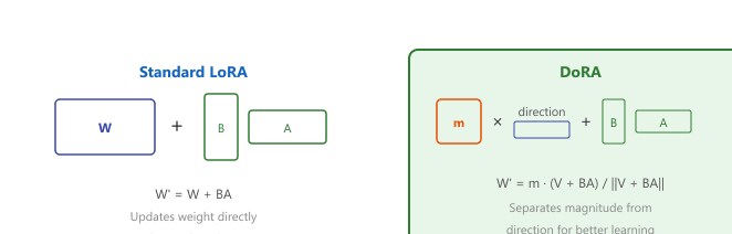
The asymmetry is mechanical, not empirical. LoRA learns ΔW = BA in a single low-rank subspace, which forces magnitude and direction updates to be entangled: scaling a column of B changes both the direction of the update and its norm. DoRA decomposes W = m · V/‖V‖ and updates the unit-direction matrix V with low-rank, while updating the magnitude vector m separately. This lets the optimizer move along the unit sphere without using rank capacity to also re-scale, so the same rank budget buys more directional expressivity. The framework generalizes the classical "decouple weight decay from gradient" trick (AdamW) one level deeper into the parameterization itself.
DoRA (2024) improves on LoRA by decomposing the pretrained weight into its magnitude and direction components before applying the low-rank update. Specifically, a weight vector w is decomposed as w = m · (w / ||w||), where m is a learnable magnitude scalar and the direction is updated via standard LoRA. This decomposition aligns more closely with how full fine-tuning actually modifies weights, resulting in better performance for the same rank.
Think of pointing a flashlight: LoRA must learn both which direction to aim and how bright the beam should be using the same dial. If you want to brighten the beam without rotating it, LoRA still has to use some of its low-rank capacity to keep the angle steady, wasting parameters. DoRA gives you two dials: one for the angle (low-rank, like LoRA) and a separate scalar for the brightness. Now the rank budget can spend all its capacity on rotation, and the magnitude scalar adjusts intensity independently. That separation is why DoRA at rank 16 typically matches LoRA at rank 32 with fewer trainable parameters.
If you are already using LoRA and want a quick accuracy boost, try switching to DoRA before increasing rank. In most benchmarks, DoRA at rank 16 outperforms LoRA at rank 32, while using fewer trainable parameters. The PEFT library supports DoRA as a drop-in replacement: just set use_dora=True in your LoraConfig.
The original DoRA paper (Liu et al., 2024) reports gains of 1-3% over LoRA across commonsense reasoning, visual-instruction, and image-text understanding tasks at matched rank and target modules, with only a marginal increase in trainable parameters (the additional magnitude vectors are tiny). Independent replications find the gap is task-dependent and sometimes within noise; the safest claim is "DoRA dominates LoRA on the original benchmark suite and is rarely worse," not that it always wins. Training speed is nearly identical to LoRA. For deployment, the quantization techniques covered later in the chapter apply equally to DoRA-adapted models; the diagram below compares the LoRA and DoRA weight-update mechanisms side by side.
Think of advanced PEFT methods as a wardrobe of accessories for the same outfit. DoRA separates direction from magnitude, like choosing both which way to point and how far to reach. Prompt tuning adds learned tokens to the input, like pinning a badge onto a jacket that changes how others perceive you. Each accessory targets a different aspect of the model's behavior, and you can mix and match them depending on the task at hand.
The following implementation (Code Fragment 17.2.3) shows how to enable DoRA with a single configuration flag.
QLoRA is the composition of two libraries: bitsandbytes for NF4 base-model quantization and peft for the LoRA adapter that trains in BF16. The glue is prepare_model_for_kbit_training, which casts norm layers back to FP32 and enables gradient checkpointing so that the 4-bit base is differentiable end-to-end. The recipe below fine-tunes a 70B model on a single 48 GB GPU.
Show code
pip install bitsandbytes peft transformers trl
from transformers import AutoModelForCausalLM, BitsAndBytesConfig
from peft import LoraConfig, get_peft_model, prepare_model_for_kbit_training
import torch
bnb = BitsAndBytesConfig(load_in_4bit=True, bnb_4bit_quant_type="nf4",
                         bnb_4bit_compute_dtype=torch.bfloat16,
                         bnb_4bit_use_double_quant=True)
base = AutoModelForCausalLM.from_pretrained("meta-llama/Llama-3.1-70B-Instruct",
                                            quantization_config=bnb, device_map="auto")
base = prepare_model_for_kbit_training(base)
model = get_peft_model(base, LoraConfig(r=16, lora_alpha=32,
                                        target_modules="all-linear",
task_type="CAUSAL_LM"))# Configure QLoRA adapter parameters on top of the quantized base
# The adapter trains in float16 while the base stays in 4-bit NormalFloat
from peft import LoraConfig, get_peft_model
# DoRA configuration: enable the use_dora flag
dora_config = LoraConfig(
r=16,
lora_alpha=32,
target_modules=[
"q_proj", "k_proj", "v_proj", "o_proj",
"gate_proj", "up_proj", "down_proj",
],
lora_dropout=0.05,
use_dora=True, # Enable DoRA
task_type="CAUSAL_LM",
)
model = get_peft_model(base_model, dora_config)
model.print_trainable_parameters()
# Slightly more params than LoRA due to magnitude vectors,
# but typically ~1-3% better accuracy at same rank.Code Fragment 17.2.6 shows how Prefix Tuning prepends learnable vectors to each attention layer.
# Prefix Tuning: prepend learnable key-value vectors to each attention layer
# The model attends to these "virtual tokens" alongside real input tokens
from peft import PrefixTuningConfig, get_peft_model, TaskType

# Prefix Tuning configuration
prefix_config = PrefixTuningConfig(
 task_type=TaskType.CAUSAL_LM,
 num_virtual_tokens=30, # Number of prefix tokens
 prefix_projection=True, # Use MLP to project prefix (more stable)
 encoder_hidden_size=1024, # Hidden size of projection MLP
)

# Wrap base model with trainable LoRA adapters
model = get_peft_model(base_model, prefix_config)
model.print_trainable_parameters()
# Typically 0.1-0.5% of total parametersprefix_projection flag enables a small MLP that projects the prefix, improving training stability. This approach modifies the model's behavior through attention steering rather than weight modification.A bottleneck adapter is the small trainable module Houlsby et al. (2019) insert after the feed-forward (and sometimes after the attention) sub-layer of each transformer block. Given a hidden state $h \in \mathbb{R}^d$, the adapter down-projects to a small bottleneck dimension $r \ll d$, applies a non-linearity, projects back to $d$, and adds the result residually:
$$h' = h + W_{\text{up}}\, \sigma\!\big(W_{\text{down}}\, h\big), \qquad W_{\text{down}} \in \mathbb{R}^{r \times d},\ W_{\text{up}} \in \mathbb{R}^{d \times r}$$
The down-up sandwich is initialised so that $W_{\text{up}} \approx 0$, which makes the adapter the identity at the start of training; gradients then carve out a per-task perturbation in the $2 d r$ parameters of $(W_{\text{down}}, W_{\text{up}})$ while the base weights stay frozen. For a 7B model with $d = 4096$ and $r = 16$, each adapter holds $\approx 131$k parameters, so a full set across 32 layers costs roughly 0.06% of the base. Code Fragment 17.2.5 demonstrates the bottleneck adapter pattern using LLaMA-Adapter style chapters, and Code Fragment 17.2.4b shows the authentic Houlsby-style configuration via the adapters library.
# Houlsby-style bottleneck adapters via the adapters library
# (the modern successor to adapter-transformers / AdapterHub).
from adapters import AutoAdapterModel, SeqBnConfig
from transformers import AutoTokenizer

model = AutoAdapterModel.from_pretrained("bert-base-uncased")
tok = AutoTokenizer.from_pretrained("bert-base-uncased")

# Sequential bottleneck: W_down (d -> r), ReLU, W_up (r -> d), residual add.
adapter_cfg = SeqBnConfig(reduction_factor=16, non_linearity="relu")
model.add_adapter("legal-clauses", config=adapter_cfg)
model.add_classification_head("legal-clauses", num_labels=3)
model.train_adapter("legal-clauses")   # freezes base, trains only the bottleneck

# Standard HF Trainer loop trains ~0.9M params on a 110M-param BERT.
Code Fragment 17.2.4b: Authentic Houlsby-style bottleneck adapter via the adapters library. SeqBnConfig instantiates the $W_{\text{up}} \sigma(W_{\text{down}} h)$ sandwich with reduction factor $r = d / 16$ and freezes the base model so only the adapter and the small classification head receive gradients.
# Adapter layers: insert small bottleneck modules between transformer layers
# Uses LLaMA-Adapter style via PEFT's AdaptionPromptConfig
from peft import AdaptionPromptConfig, get_peft_model

# Note: For bottleneck adapters, use the adapters library
# from adapters import AutoAdapterModel

# Example with LLaMA-Adapter style (via PEFT)
adapter_config = AdaptionPromptConfig(
 adapter_len=10, # Length of adapter prompt
 adapter_layers=30, # Number of layers to add adapters
 task_type="CAUSAL_LM",
)

model = get_peft_model(base_model, adapter_config)
model.print_trainable_parameters()The bottleneck adapter pattern (down-project to a small dimension, non-linearity, up-project, residual add) predates LoRA: it was introduced by Houlsby et al. (2019) and refined by Pfeiffer et al. (2020) into the modules curated by AdapterHub, the original library of pretrained PEFT modules for BERT-era encoder models. AdapterHub catalogues hundreds of task and language adapters that can be loaded, stacked, and "AdapterFusion"-combined without any retraining of the base model. While LoRA has displaced bottleneck adapters as the default PEFT choice for modern decoder LLMs, the AdapterHub ecosystem remains the canonical reference for encoder-style multi-task adapter routing and is the historical reason the umbrella term "adapter" is so overloaded in the literature.
17.2.2 IA3: Infused Adapter by Inhibiting and Amplifying Inner Activations
IA3 (few-shot parameter-efficient fine-tuning Is All You Need, 2022) takes parameter efficiency to the extreme. Instead of learning new matrices or inserting new layers, IA3 learns only three rescaling vectors that modulate the keys, values, and intermediate activations in the Transformer architecture. The total number of trainable parameters is typically 10x smaller than LoRA.
The tradeoff is that IA3's limited capacity makes it best suited for simple adaptation tasks (format changes, style transfer) rather than complex domain adaptation. It excels in few-shot settings where overfitting is a concern. Code Fragment 17.2.6a demonstrates IA3 configuration.
# IA3 configuration: learns only rescaling vectors
# Extreme parameter efficiency at the cost of limited adaptation capacity
from peft import IA3Config, get_peft_model, TaskType

ia3_config = IA3Config(
 task_type=TaskType.CAUSAL_LM,
 target_modules=["k_proj", "v_proj", "down_proj"],
 feedforward_modules=["down_proj"],
)

# Wrap base model with IA3 rescaling vectors
model = get_peft_model(base_model, ia3_config)
model.print_trainable_parameters()
# trainable params: ~500K for a 7B model (0.007%)VeRA (Kopiczko et al., 2024, arXiv:2310.11454) pushes LoRA's parameter count an order of magnitude lower. Instead of learning a separate low-rank A and B per layer, VeRA FREEZES a single pair of random matrices A and B that are SHARED across all adapted layers and never updated; the only trainable parameters are two small diagonal scaling vectors b and d per layer, giving the update Delta W = diag(b) B diag(d) A. Because the random projections are fixed and shared, storage per task collapses to a few vectors, while the learned scalings still let each layer select and rescale directions in the random subspace. VeRA matches LoRA on many tasks at a fraction of the trainable parameters, useful when serving thousands of per-user adapters.
17.2.3 Comprehensive PEFT Method Comparison
| Method | Params (%) | Memory | Inference Overhead | Best For |
|---|---|---|---|---|
| LoRA | 0.1-0.5% | Low | Zero (after merge) | General purpose, most tasks |
| QLoRA | 0.1-0.5% | Very Low | Zero (after merge) | Large models on limited GPU |
| DoRA | 0.1-0.5% | Low | Zero (after merge) | When LoRA quality is insufficient |
| LoRA+ | 0.1-0.5% | Low | Zero (after merge) | Faster convergence needed |
| Prefix Tuning | 0.1-0.5% | Low | Small (longer KV cache) | NLU tasks, multi-task serving |
| Prompt Tuning | <0.01% | Very Low | Negligible | Very large models, simple tasks |
| Adapters | 0.5-3% | Medium | Small (sequential) | Compositional multi-task |
| IA3 | <0.01% | Very Low | Negligible | Few-shot, style adaptation |
Prompt Tuning and IA3 achieve extreme parameter efficiency, but they are significantly less capable than LoRA for complex adaptation tasks. If your task requires learning new knowledge (domain-specific terminology, code patterns, specialized reasoning), LoRA or DoRA with a reasonable rank (16-64) will substantially outperform these lighter methods. Reserve IA3 and Prompt Tuning for scenarios where simplicity or parameter count is the primary constraint.
Why this matters: The proliferation of PEFT methods (DoRA, AdaLoRA, IA3, GaLore) is not just academic variety; each addresses a specific limitation of vanilla LoRA. DoRA handles magnitude-direction decomposition for better convergence. AdaLoRA allocates rank adaptively, putting more parameters where they help most. IA3 achieves extreme parameter efficiency (orders of magnitude fewer parameters than LoRA) at the cost of some task performance. The practical guidance is: start with standard LoRA, and only explore these variants when you have a specific bottleneck (convergence issues, memory constraints, or multi-task serving requirements).
17.2.4 Multi-Adapter Serving
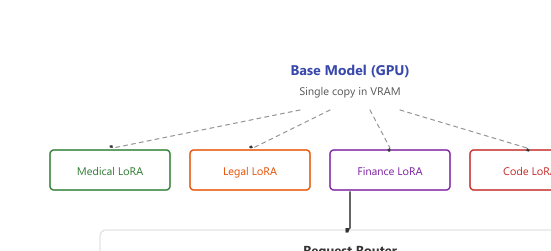
One of LoRA's most powerful production features is the ability to serve many adapters from a single base model. This enables multi-tenant deployments where each customer or task gets its own fine-tuned behavior without duplicating the base model weights, a significant advantage for inference optimization. Two main systems support this at scale: LoRAX (formerly LoRAX by Predibase) and S-LoRA.
17.2.4.1 Architecture Overview
Figure 17.2.2a illustrates how a single base model serves multiple LoRA adapters dynamically at request time.
17.2.4.2 LoRAX and S-LoRA
LoRAX (Predibase) is a production-grade serving system that can host hundreds of fine-tuned LoRA adapters on a single GPU. It keeps the base model in GPU memory and dynamically loads adapter weights per request. Key features include adapter weight caching, batched inference across different adapters, and automatic adapter management.
S-LoRA (from UC Berkeley) takes a more research-oriented approach, using unified paging to manage adapter memory and custom CUDA kernels for batched LoRA computation. S-LoRA can serve thousands of adapters simultaneously, with adapters stored in a tiered memory system (GPU, CPU, disk) and paged in on demand.
Multi-adapter serving is one of the strongest arguments for LoRA over other PEFT methods in production. A single A100 GPU can serve a base 7B model with hundreds of LoRA adapters, effectively providing hundreds of specialized models at the cost of one. This is far more economical than deploying separate merged models for each use case.
Who: Daniela, a platform architect at a B2B content-generation SaaS company.
Situation: The company had 50 enterprise customers, each requiring a specialized writing style (tone, vocabulary, formatting conventions) for their generated marketing copy. The product ran on a 7B-parameter base model.
Problem: Deploying 50 separate fine-tuned models would require 50 GPUs, pushing monthly infrastructure costs above $150,000. The engineering team also dreaded maintaining 50 independent model deployments, each with its own versioning and rollback pipeline.
Decision: Daniela trained 50 lightweight LoRA adapters (each roughly 20 MB) and served them all from a single A100 using LoRAX. Per-request routing attached the correct adapter based on the customer's API key, and new customer onboarding required only a fresh LoRA training run (under two hours on one GPU).
Result: Total GPU cost dropped from 50 instances to one A100, a roughly 98% cost reduction. New adapters slotted into the shared serving infrastructure with zero downtime. Median response latency increased by only 8ms compared to a dedicated model, which was imperceptible to end users.
Lesson: For multi-tenant serving where each customer needs a specialized model, LoRA adapters plus a shared base model eliminate the linear scaling of GPU costs with customer count. The key enabler is adapter hot-swapping at the serving layer.
17.2.5 Choosing the Right PEFT Method
With so many PEFT options available, the decision can feel overwhelming. Here is a practical decision framework based on your constraints and requirements.
| Scenario | Recommended Method | Reasoning |
|---|---|---|
| General fine-tuning (default) | LoRA (r=16) | Best quality/efficiency tradeoff, widest ecosystem support |
| Limited GPU memory | QLoRA | 4-bit base model frees VRAM for larger models or batches |
| Need extra quality over LoRA | DoRA | Drop-in upgrade, consistent 1-3% improvement |
| Training speed is critical | LoRA+ | 1.5-2x faster convergence, same final quality |
| Multi-tenant serving (100+ tasks) | LoRA + LoRAX | Hot-swappable adapters from single base |
| Extreme parameter budget (<1K params) | IA3 | Learns only rescaling vectors, minimal overfitting |
| Very large model (100B+), simple task | Prompt Tuning | Ultra-lightweight, scales well with model size |
| NLU classification tasks | Prefix Tuning | Strong at steering attention for classification |
When in doubt, start with LoRA. It has the widest library support, the most documentation, and works well across virtually all tasks and model sizes. Move to specialized methods only when you have a specific constraint (memory, serving architecture, parameter count) that LoRA cannot satisfy.
17.2.6 GaLore: Gradient Low-Rank Projection
While LoRA reduces the number of trainable parameters by adding low-rank adapters, GaLore (Gradient Low-Rank Projection) takes a fundamentally different approach: it reduces optimizer memory by projecting gradients into a low-rank subspace. This distinction matters because optimizer states (momentum and variance in Adam) typically consume two to three times the memory of the parameters themselves. GaLore enables full-parameter training of large models on consumer hardware, something that LoRA alone cannot achieve because LoRA still freezes the base model and only updates the adapter.
17.2.6.1 How GaLore Works
During training, GaLore periodically computes the SVD of the gradient matrix for each weight layer, retaining only the top-r singular vectors. The optimizer states (Adam's first and second moments) are maintained in this reduced r-dimensional space rather than the full parameter space. Every T steps (typically T=200), the projection matrices are recomputed from the current gradient to track the evolving optimization landscape. The key insight is that gradient matrices during LLM training tend to be approximately low-rank, so very little information is lost by this projection. Code Fragment 17.2.7 provides a conceptual implementation.
# GaLore conceptual implementation
import torch

class GaLoreProjector:
    """Project gradients to low-rank subspace for memory-efficient training."""
    def __init__(self, rank: int, update_freq: int = 200):
        self.rank = rank
        self.update_freq = update_freq
        self.step = 0
        self.projector = None

    def project(self, grad: torch.Tensor) -> torch.Tensor:
        """Project full gradient to low-rank subspace."""
        if self.step % self.update_freq == 0:
            # Recompute projection via SVD
            U, S, Vh = torch.linalg.svd(grad, full_matrices=False)
            self.projector = U[:, :self.rank]
        self.step += 1
        # Project gradient: (d, r) @ (r, d) is never formed explicitly
        return self.projector.T @ grad  # shape: (rank, d_out)

    def back_project(self, low_rank_update: torch.Tensor) -> torch.Tensor:
        """Map low-rank update back to full parameter space."""
        return self.projector @ low_rank_update
In practice, the galore_torch library wraps this into a drop-in optimizer replacement:
# Library shortcut: GaLore optimizer (pip install galore-torch)
from galore_torch import GaLoreAdamW8bit
optimizer = GaLoreAdamW8bit(
    model.parameters(),
    lr=1e-5,
    rank=128, # low-rank projection dimension
    update_proj_gap=200, # recompute SVD every 200 steps
)
# Use this optimizer in any standard training loop; no other changes needed.GaLoreAdamW8bit optimizer handles SVD projection, subspace tracking, and 8-bit quantization of optimizer states internally. Replace your standard optimizer with this single line to enable full-parameter training on consumer GPUs.The memory savings are substantial. For a 7B parameter model, standard Adam requires roughly 42 GB of optimizer state memory (two copies of all parameters in float32). With GaLore at rank 128, the optimizer states shrink to approximately 2 to 4 GB, enabling full-parameter training of 7B models on a single 24 GB GPU. The authors demonstrated that GaLore can pretrain LLaMA models up to 7B parameters on a single GPU with no loss in quality compared to full-rank Adam.
GaLore and LoRA solve different problems. LoRA reduces the number of trainable parameters by adding small adapters. GaLore reduces optimizer memory by projecting gradients into a low-rank space while still updating all parameters. You can combine both: use GaLore for pretraining data or full fine-tuning, and LoRA for lightweight adaptation where you want a modular, hot-swappable adapter.
17.2.7 rsLoRA: Rank-Stabilized LoRA
Standard LoRA initializes the low-rank matrices A and B such that the adapter output is scaled by a fixed factor α/r, where α is a hyperparameter and r is the rank. This scaling creates a practical problem: when you change the rank, the effective magnitude of the adapter's contribution changes, requiring you to re-tune the learning rate and α for each rank setting. This makes rank selection tedious and error-prone.
rsLoRA (rank-stabilized LoRA) addresses this by changing the scaling factor from α/r to α/√r. This seemingly small modification has a significant theoretical and practical impact. The √r scaling ensures that the adapter's output magnitude remains stable as the rank changes, because the variance of the product BA scales proportionally with r under random initialization. With α/√r scaling, doubling the rank does not double the adapter's contribution; it increases it by only √2, which is the correct normalization for maintaining stable training dynamics. Code Fragment 17.2.7b compares the two scaling approaches.
# rsLoRA vs standard LoRA scaling comparison
import torch
import math
def lora_forward(x, A, B, alpha, rank, use_rslora=False):
    """Compare standard LoRA and rsLoRA scaling."""
    lora_output = x @ A @ B # shape: (batch, d_out)
    if use_rslora:
        # rsLoRA: scale by alpha / sqrt(rank)
        scaling = alpha / math.sqrt(rank)
    else:
        # Standard LoRA: scale by alpha / rank
        scaling = alpha / rank
    return lora_output * scaling

# Demonstrate stability across ranks
d_in, d_out, alpha = 4096, 4096, 16.0
x = torch.randn(1, d_in)
for rank in [4, 16, 64, 256]:
    A = torch.randn(d_in, rank) * 0.01
    B = torch.randn(rank, d_out) * 0.01
    std_out = lora_forward(x, A, B, alpha, rank, use_rslora=False)
    rs_out = lora_forward(x, A, B, alpha, rank, use_rslora=True)
    print(f"rank={rank:3d} standard_norm={std_out.norm():.4f}"
f" rslora_norm={rs_out.norm():.4f}")The practical benefit is straightforward: with rsLoRA, you can change the rank without retuning other hyperparameters. A learning rate and α that work well at rank 16 will also work well at rank 64 or rank 256. This makes hyperparameter search much faster (complementing the training loop fundamentals from Section 16.3), because you can tune the learning rate at a low rank (which trains quickly) and then scale up the rank for higher quality without adjusting anything else. rsLoRA is available in PEFT via the use_rslora=True parameter in LoraConfig.
| Property | Standard LoRA | rsLoRA | GaLore |
|---|---|---|---|
| What it optimizes | Parameter count | Parameter count | Optimizer memory |
| Scaling factor | α/r | α/√r | N/A (full params) |
| Rank-stable? | No (retune per rank) | Yes | Yes |
| Updates base weights? | No (adapter only) | No (adapter only) | Yes (all params) |
| Typical use case | Fine-tuning | Fine-tuning | Pretraining, full fine-tuning |
| Library support | PEFT, Unsloth | PEFT (use_rslora=True) | galore-torch, PEFT |
rsLoRA is a drop-in improvement with no computational overhead. If you are using PEFT's LoraConfig, add use_rslora=True and your adapter scaling will be rank-stable. There is no reason not to enable it for any new LoRA training run. GaLore requires more setup (a custom optimizer) but enables training regimes that are otherwise impossible on limited hardware.
Applying LoRA to only the attention layers (q_proj, v_proj) is the classic default, but recent research shows targeting all linear layers (including MLP) gives better results for a modest increase in trainable parameters. Try target_modules="all-linear" in PEFT.
The PEFT method zoo has grown so large that researchers now publish "survey of survey" papers just to catalog them all. At last count, the literature contained over 40 distinct PEFT variants, many named with creative acronyms: LoRA, DoRA, QLoRA, rsLoRA, LoRA+, AdaLoRA, LoHa, LoKr, OFT, BOFT, VeRA, IA3, and more. Some researchers joke that the field has more LoRA variants than there are letters in the alphabet. The good news: despite this Cambrian explosion, about 90% of practitioners use plain LoRA or QLoRA, and that is perfectly fine for most tasks.
Unified PEFT frameworks are emerging that combine adapter insertion, soft prompt tuning, and low-rank decomposition into a single configurable system, allowing automated search over PEFT method combinations. Research on (IA)^3 demonstrates that learning just three rescaling vectors per layer can match LoRA performance with even fewer parameters. The frontier challenge is developing PEFT methods that work reliably for multimodal models (vision-language, audio-language), where optimal adapter placement differs from text-only transformers.
Recent work on mixture-of-LoRA-experts (2024) routes inputs to specialized LoRA adapters using a learned gating mechanism, combining the modularity of multi-adapter serving with the capacity of larger models.
- DoRA improves LoRA by decomposing weights into magnitude and direction, yielding 1-3% gains with a single configuration flag (
use_dora=True). - LoRA+ accelerates convergence by using asymmetric learning rates for A and B matrices, saving training compute without sacrificing quality.
- Prefix Tuning prepends learnable key-value pairs to every attention layer, offering an alternative to weight modification that works well for NLU tasks.
- Prompt Tuning is the most parameter-efficient method (<0.01%), but is only competitive with very large models and simple tasks.
- IA3 learns only rescaling vectors, achieving extreme parameter efficiency at the cost of limited adaptation capacity.
- Multi-adapter serving (LoRAX, S-LoRA) lets you host hundreds of specialized models on a single GPU by hot-swapping LoRA adapters per request.
- When in doubt, use LoRA. It has the best ecosystem support, works across all model sizes and task types, and can be upgraded to DoRA or LoRA+ with minimal changes.
Show Answer
use_dora=True. Prefer DoRA when you want a free 1-3% accuracy improvement with minimal extra cost over standard LoRA.Show Answer
Show Answer
Show Answer
Show Answer
Exercises
Explain how DoRA (Weight-Decomposed Low-Rank Adaptation) improves on standard LoRA. What is the magnitude-direction decomposition?
Answer Sketch
DoRA decomposes each weight matrix into a magnitude component (scalar per column) and a direction component (unit vector). LoRA is then applied only to the direction component, while the magnitude is learned separately. This mirrors how full fine-tuning naturally adjusts both magnitude and direction. Standard LoRA couples these two, making it harder to learn the right balance. DoRA typically improves accuracy by 1 to 3% over LoRA with minimal additional overhead.
Describe how prefix tuning works. How does prepending learned 'virtual tokens' to the input differ from manual prompt engineering?
Answer Sketch
Prefix tuning prepends a sequence of learned continuous vectors (virtual tokens) to each layer's key and value representations. Unlike manual prompt engineering (which uses discrete text tokens), prefix tuning optimizes in continuous space, allowing the model to find representations that no natural language token could express. The virtual tokens are trained via backpropagation while the model is frozen. Prefix tuning modifies the attention pattern without changing any model weights.
IA3 learns only three rescaling vectors per layer. Calculate the total number of trainable parameters for a 7B model with 32 layers, where each layer has hidden dimension 4096.
Answer Sketch
IA3 learns three vectors per layer: one for keys (d=4096), one for values (d=4096), and one for the FFN intermediate layer (d=11008 for Llama). Per layer: 4096 + 4096 + 11008 = 19,200 parameters. Total: 32 * 19,200 = 614,400 parameters. For a 7B model, this is 0.009% of total parameters. Compare to LoRA rank 16: ~10M parameters (0.14%). IA3 is 16x more parameter-efficient than LoRA but may sacrifice adaptation quality for complex tasks.
You need to fine-tune a single base model for 50 different customer tenants, each with unique data. Which PEFT method would you choose, and why?
Answer Sketch
LoRA is ideal for multi-tenant serving. Each tenant gets their own small adapter (~10 to 50MB) that can be hot-swapped at inference time without reloading the base model (~14GB for 7B). Frameworks like LoRAX and S-LoRA serve hundreds of adapters from a single GPU. Prefix tuning is an alternative but adds serving latency. Full fine-tuning would require 50 separate model copies (700GB+). LoRA gives per-tenant customization at 1/300th the storage cost.
Write the key code to add a soft prompt (10 learned tokens) to a model using the PEFT library's PromptTuningConfig. Include model loading, config setup, and training.
Answer Sketch
Config: config = PromptTuningConfig(task_type='CAUSAL_LM', num_virtual_tokens=10, prompt_tuning_init='RANDOM'). Apply: model = get_peft_model(model, config). The model now has 10 * hidden_dim trainable parameters (e.g., 10 * 4096 = 40,960 for Llama-7B). Train normally with any SFT trainer. At inference, the learned soft prompt is prepended automatically. Total trainable parameters: 0.0006% of the model.
What Comes Next
In the next section, Section 17.3: Training Platforms & Tools, we cover training platforms and tools, the practical infrastructure for running PEFT workflows at scale.