I taught my model legal documents on Monday and it forgot how to write code by Friday. Catastrophic forgetting is the most polite name we have for "the bill came due."
Distill, Catastrophically-Forgetting AI Agent
LLMs are expensive to pretrain and quickly become outdated. New knowledge emerges, domains evolve, and organizational needs change. Continual learning addresses how to update a model with new information without expensive retraining from scratch, while avoiding "catastrophic forgetting" of previously learned capabilities. This section covers continual pretraining data on domain corpora, vocabulary extension for specialized terminology, replay methods, regularization techniques like Elastic Weight Consolidation, and progressive training strategies. These methods are essential for maintaining production LLMs that must adapt to changing requirements over time. The fine-tuning fundamentals from Section 16.1 provide the baseline adaptation spectrum that continual learning extends.
Prerequisites
This section assumes familiarity with fine-tuning fundamentals from Section 16.2 (including catastrophic forgetting in full fine-tuning) and the LoRA adapter approach from Section 17.1. You should also understand model merging from Section 17.7, as adapter merging is a key strategy for composable domain adaptation.
The crossing-curves dynamic shown for fine-tuning in Figure 17.8.1 applies identically to continual learning. As domain performance climbs, general capabilities decline; the goal is to find and maintain the sweet spot. The same chart and the same intervention strategies (replay, distillation, careful LR scheduling) apply.
Catastrophic forgetting is more severe in full fine-tuning than in parameter-efficient methods. LoRA naturally mitigates forgetting because the base model weights remain frozen, and the low-rank adapter can only make limited modifications. This is one reason why LoRA-based continual learning is increasingly preferred over full-parameter continual pretraining for domain adaptation.
Who: AI team at a financial services firm
Situation: The team adapted Llama-2 13B for financial analysis, but quarterly regulation changes and new financial instruments required regular model updates.
Problem: Each full fine-tuning cycle on updated data caused catastrophic forgetting: the model lost 15% accuracy on previously learned SEC filing formats while learning new ones.
Dilemma: Retraining from scratch on all historical plus new data was prohibitively expensive (72 GPU-hours per cycle), but incremental training on only new data caused severe forgetting.
Decision: They adopted elastic weight consolidation (EWC) combined with LoRA adapters, using replay buffers containing 10% of historical examples mixed into each update batch.
How: The Fisher information matrix identified which weights were critical for existing knowledge. EWC penalized changes to those weights during updates. A replay buffer of 2,000 curated examples from each previous quarter was mixed into training data.
Result: Forgetting dropped from 15% to under 2% accuracy loss on old tasks. Each quarterly update required only 8 GPU-hours (89% reduction), and the model maintained 94% accuracy across all historical and new regulation formats.
Lesson: Combining parameter-efficient methods (LoRA) with explicit anti-forgetting techniques (EWC + replay) is far more effective than either approach alone for ongoing model updates.
Why this matters: Continual learning is the production reality of deployed models. Knowledge becomes outdated, regulations change, new products launch, and user behavior shifts. A model fine-tuned in January may be subtly wrong by June. The techniques in this section (replay buffers, elastic weight consolidation, progressive training) are not theoretical curiosities; they are the infrastructure for keeping models current without retraining from scratch. This connects to the broader drift monitoring strategies in Chapter 29, where detecting when a model needs updating is just as important as knowing how to update it.
Continual pretraining is the recipe behind several public domain-specific LLMs. BloombergGPT (50B params, 2023) was trained by mixing 363B tokens of financial text with general data and is the canonical CPT case study. Meditron (Llama-2 70B continually pretrained on medical literature by EPFL) and Google's Med-PaLM show the same pattern in healthcare. StarCoder2 (the Hugging Face / BigCode collaboration) starts from a general checkpoint and continues pretraining on 600+ programming languages. The trick across all three: a small replay fraction (5 to 20 percent) of the original pretraining mix is interleaved with domain data to limit catastrophic forgetting of general capabilities.
17.8.2 Continual Pre-Training
Continual pretraining (CPT) extends the standard pretraining objective (next-token prediction) on domain-specific corpora. Unlike instruction fine-tuning, which teaches the model to follow a new format, CPT injects new factual knowledge and domain vocabulary into the model's weights. This is the primary technique for creating domain-specific foundation models (for example, a medical LLM or a financial LLM). Code Fragment 17.8.5 demonstrates the data preparation step for CPT.
17.8.2.1 Data Preparation for CPT
This snippet prepares a domain-specific corpus for continued pretraining by tokenizing and chunking the text.
# Load evaluation datasets for comparing distilled vs. base models
# Use held-out test sets that neither model saw during training
from datasets import load_dataset, concatenate_datasets
from transformers import AutoTokenizer
import random

def prepare_cpt_dataset(
    domain_data_path: str,
    general_data_path: str,
    replay_ratio: float = 0.1,
    tokenizer_id: str = "meta-llama/Meta-Llama-3-8B",
    max_seq_length: int = 4096,
    ):
    """Prepare CPT dataset with replay data to reduce forgetting."""
    tokenizer = AutoTokenizer.from_pretrained(tokenizer_id)

    # Load domain-specific data
    domain_ds = load_dataset("text", data_files=domain_data_path, split="train")
    print(f"Domain data: {len(domain_ds)} documents")

    # Load general replay data (subset of original pretraining mix)
    general_ds = load_dataset("text", data_files=general_data_path, split="train")

    # Sample replay data proportionally
    n_replay = int(len(domain_ds) * replay_ratio)
    general_ds = general_ds.shuffle(seed=42).select(range(min(n_replay, len(general_ds))))
    print(f"Replay data: {len(general_ds)} documents ({replay_ratio*100:.0f}%)")

    # Combine and shuffle
    combined = concatenate_datasets([domain_ds, general_ds])
    combined = combined.shuffle(seed=42)

    # Tokenize
def tokenize(examples):
    return tokenizer(
        examples["text"],
        truncation=True,
        max_length=max_seq_length,
        padding=False,
        )

    tokenized = combined.map(tokenize, batched=True, remove_columns=["text"])
    return tokenized
per-param penalties: [0.9 0.001]
total EWC penalty: 450.5
Code Fragment 17.8.4 defines training hyperparameters.
# Load both the teacher and student models for side-by-side evaluation
# Measure accuracy, latency, and memory footprint for each
from transformers import (
 AutoModelForCausalLM, AutoTokenizer,
 TrainingArguments, Trainer, DataCollatorForLanguageModeling
)
import torch

# Load base model
model = AutoModelForCausalLM.from_pretrained(
 "meta-llama/Meta-Llama-3-8B",
 torch_dtype=torch.bfloat16,
 device_map="auto",
)
# Load tokenizer with vocabulary matching the model
tokenizer = AutoTokenizer.from_pretrained("meta-llama/Meta-Llama-3-8B")
tokenizer.pad_token = tokenizer.eos_token

# CPT-specific training arguments
training_args = TrainingArguments(
 output_dir="./cpt-medical-llama",
 num_train_epochs=1, # Typically 1-2 epochs for CPT
 per_device_train_batch_size=4,
 gradient_accumulation_steps=8, # Effective batch size = 32
 learning_rate=2e-5, # Much lower than pre-training
 lr_scheduler_type="cosine",
 warmup_ratio=0.05,
 weight_decay=0.1,
 bf16=True,
 logging_steps=50,
 save_strategy="steps",
 save_steps=500,
 max_grad_norm=1.0,
)

data_collator = DataCollatorForLanguageModeling(
 tokenizer=tokenizer, mlm=False # Causal LM (next-token prediction)
)

# Initialize HuggingFace Trainer with model, data, and config
trainer = Trainer(
 model=model,
 args=training_args,
 train_dataset=cpt_dataset,
 data_collator=data_collator,
)

# Launch the training loop
trainer.train()
Code Fragment 17.8.5a below implements a replay-aware dataset class that interleaves domain and general examples.
# Replay dataset: mix domain data with general replay samples
# Interleaving prevents clustering of replay data at batch boundaries
from torch.utils.data import Dataset, DataLoader
import random

class ReplayDataset(Dataset):
    """Dataset that mixes domain data with replay data."""

    def __init__(self, domain_dataset, replay_dataset, replay_ratio=0.1):
        self.domain = domain_dataset
        self.replay = replay_dataset
        self.replay_ratio = replay_ratio

        # Calculate sizes for interleaving
        self.total_size = len(domain_dataset)
        self.n_replay_per_epoch = int(self.total_size * replay_ratio)

        # Pre-sample replay indices for this epoch
        self._resample_replay()

    def _resample_replay(self):
        """Resample replay indices (call at each epoch start)."""
        replay_indices = random.sample(
            range(len(self.replay)),
            min(self.n_replay_per_epoch, len(self.replay))
            )
        # Interleave: every ~(1/ratio) steps, insert a replay sample
        self.schedule = []
        replay_iter = iter(replay_indices)
        interval = int(1 / self.replay_ratio) if self.replay_ratio > 0 else 999999
        for i in range(self.total_size):
            self.schedule.append(("domain", i))
            if (i + 1) % interval == 0:
                try:
                    self.schedule.append(("replay", next(replay_iter)))
                except StopIteration:
                    pass

            def __len__(self):
                return len(self.schedule)

            def __getitem__(self, idx):
                source, data_idx = self.schedule[idx]
                if source == "domain":
                    return self.domain[data_idx]
                else:
return self.replay[data_idx]17.8.3 Elastic Weight Consolidation (EWC)
Elastic Weight Consolidation (Kirkpatrick et al., 2017) adds a regularization term to the loss function that penalizes changes to parameters that were important for previous tasks. It estimates each parameter's "importance" using the Fisher Information Matrix, which measures how much the loss changes when a parameter is perturbed. Important parameters get a stronger regularization penalty, anchoring them near their original values while allowing less important parameters to adapt freely.
The "why" behind the Fisher anchor. A flat L2 penalty (anchor every parameter equally) would freeze the model: domain learning competes uniformly with task-A knowledge and you cannot adapt. EWC's insight is that loss landscapes are not isotropic, the loss is steep in some directions (small perturbation, big damage to task A) and almost flat in others (large perturbation, no effect). The diagonal Fisher is exactly the local curvature in each direction, so weighting the penalty by Fi gives you a per-parameter spring constant: parameters that lie in a narrow valley for task A get stiff springs (cannot move), while parameters in flat regions move freely to learn task B. This is a second-order Bayesian-flavored regularizer wearing a deceptively simple quadratic suit.
As shows, the strength of each "rubber band" is proportional to the parameter's Fisher information score, creating a selective constraint that protects critical knowledge while allowing the model to learn.
The EWC loss adds a quadratic penalty term:
where $F_{i}$ is the Fisher information for parameter $i$, $\theta_{i}^{*}$ is the original parameter value, and $\lambda$ controls the regularization strength.
A concrete example with two parameters illustrates the selective penalty:
# EWC penalty: numeric walkthrough with two parameters
import numpy as np
theta_star = np.array([0.5, 1.2]) # original values after task A
theta_new = np.array([0.8, 1.3]) # current values during task B training
F = np.array([10.0, 0.1]) # Fisher information (importance)
lam = 1000
penalty = (lam / 2) * np.sum(F * (theta_new - theta_star) ** 2)
per_param = F * (theta_new - theta_star) ** 2
print(f"per-param penalties: {per_param}") # [0.9, 0.001]
print(f"total EWC penalty: {penalty:.1f}") # 450.5
# Parameter 1 (F=10.0) dominates: even a small shift of 0.3 costs 0.9.
# Parameter 2 (F=0.1) can move freely because it was unimportant for task A.Code Fragment 17.8.6 shows this in practice.
# Evaluate the distilled model on downstream tasks using PyTorch
# Compute accuracy, F1, and per-class metrics
import torch
import torch.nn as nn
from copy import deepcopy

class EWCRegularizer:
    """Elastic Weight Consolidation for continual learning."""

    def __init__(self, model, dataloader, device, n_samples=200):
        self.params = {
            n: p.clone().detach()
            for n, p in model.named_parameters()
            if p.requires_grad
            }
        self.fisher = self._compute_fisher(model, dataloader, device, n_samples)

    def _compute_fisher(self, model, dataloader, device, n_samples):
        """Estimate diagonal Fisher Information Matrix."""
        fisher = {
            n: torch.zeros_like(p)
            for n, p in model.named_parameters()
            if p.requires_grad
            }

        model.eval()
        count = 0
        for batch in dataloader:
            if count >= n_samples:
                break
                input_ids = batch["input_ids"].to(device)
                outputs = model(input_ids=input_ids, labels=input_ids)
                loss = outputs.loss
                loss.backward()

                for n, p in model.named_parameters():
                    if p.requires_grad and p.grad is not None:
                        fisher[n] += p.grad.detach() ** 2

                        model.zero_grad()
                        count += input_ids.size(0)

                        # Normalize
                        for n in fisher:
                            fisher[n] /= count

                            return fisher

        def penalty(self, model, lambda_ewc=1000):
            """Compute EWC regularization penalty."""
            loss = 0
            for n, p in model.named_parameters():
                if n in self.fisher:
                    loss += (self.fisher[n] * (p - self.params[n]) ** 2).sum()
                    return (lambda_ewc / 2) * loss

                    # Usage in training loop:
                        # ewc = EWCRegularizer(model, general_dataloader, device)
                        # for batch in domain_dataloader:
# loss = model(**batch).loss + ewc.penalty(model)Computing the full Fisher Information Matrix for a billion-parameter model is prohibitively expensive. In practice, EWC uses a diagonal approximation (only the diagonal of the Fisher matrix), which can be computed efficiently with a single pass over a small dataset. The lambda_ewc hyperparameter typically ranges from 100 to 10000 and requires tuning. Too low and forgetting persists; too high and the model cannot adapt to the new domain.
Elastic Weight Consolidation is the neural network equivalent of putting "do not erase" signs on a whiteboard. New information fills the empty spaces freely, but the critical notes are preserved. The Fisher information matrix is the survey that identifies which notes are critical: the bigger the Fisher value, the bigger the sign.
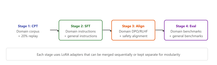
17.8.4 Progressive Training and Curriculum Approaches
Progressive training structures the continual learning process as a sequence of carefully designed stages, each building on the previous one. Rather than training on all domain data at once, you create a curriculum that gradually shifts the distribution from general to domain-specific.
The diagram below illustrates this staged approach. The subsections below detail the pipeline stages and the curriculum design principles that govern each transition.
17.8.4.1 Multi-Stage Domain Adaptation Pipeline
The diagram below traces the progressive adaptation pipeline from general to domain-specific capabilities.
17.8.4.2 Curriculum Design Principles
Effective curriculum design for continual learning follows several principles. Start with data that is closest to the original pretraining distribution and gradually shift toward the target domain. Within the domain data, present easier examples first (shorter texts, simpler concepts) and progress to harder examples. This gradual transition gives the model time to adjust its internal representations without abrupt distribution shifts.
| Strategy | Description | When to Use |
|---|---|---|
| Data mixing schedule | Start with 50% general / 50% domain, end with 10% / 90% | Large domain shift |
| Learning rate warmup | Start very low (1e-6), gradually increase to target LR | Preventing early destabilization |
| Layer-wise learning rates | Lower LR for early layers, higher for later layers | Preserving foundational features |
| LoRA rank scheduling (Sec 17.1.3.1) | Start with low rank (4), increase to final rank (16-32) | Memory-constrained setups |
| Multi-epoch curriculum | Epoch 1: easy domain data; Epoch 2: hard domain data | Diverse difficulty levels in domain |
The most practical approach to continual domain adaptation for most teams is: use LoRA (not full fine-tuning) for each adaptation stage, keep the base model frozen, and maintain a library of composable adapters. This sidesteps catastrophic forgetting entirely because the base weights never change. You can then merge adapters using the techniques from Section 17.7 to combine capabilities, or swap them dynamically at serving time.
After model merging (TIES, DARE, or linear interpolation), test on benchmarks for each source model's specialty. Merging can create subtle capability regressions that only appear on specific task types.
Continual learning for LLMs is advancing through replay-based methods that mix small amounts of previous task data into new training batches, significantly reducing catastrophic forgetting with minimal storage overhead. Research on model editing (like ROME and MEMIT) enables targeted knowledge updates to specific facts without retraining, complementing broader domain adaptation approaches.
The frontier challenge is building models that can learn continuously from deployment feedback while maintaining RLHF properties established during initial training.
- Catastrophic forgetting degrades general capabilities when training on domain data. The severity increases with training duration and is worse for full fine-tuning than for parameter-efficient methods.
- Continual pretraining uses next-token prediction on domain corpora to inject new knowledge. Use a lower learning rate (1e-5 to 5e-5) and limit to 1-2 epochs to balance adaptation and retention.
- Replay methods mix general-domain data into the training stream. A 10-20% replay ratio prevents most forgetting for typical domain adaptation scenarios.
- Vocabulary extension improves efficiency for domain-specific terminology, but requires continued training for new embeddings to become effective.
- Elastic Weight Consolidation penalizes changes to important parameters using Fisher Information, providing a principled regularization approach that does not require storing replay data.
- Progressive training structures adaptation as a multi-stage pipeline (CPT, SFT, alignment, evaluation) with curriculum-based data scheduling.
- LoRA-based adaptation is often the best practical choice because frozen base weights eliminate forgetting entirely, and adapters can be composed or swapped for modular domain specialization.
- Always evaluate on both domain and general benchmarks after continual learning to verify that domain gains have not come at the cost of general degradation.
Show Answer
Show Answer
Show Answer
Show Answer
Show Answer
Exercises
Explain two mechanisms by which catastrophic forgetting occurs during continual learning. Why does fine-tuning on new data degrade performance on old tasks?
Answer Sketch
Mechanism 1: Weight overwriting: gradient updates for the new task move shared weights away from values that were optimal for old tasks. Mechanism 2: Representation drift: the internal feature representations shift to favor the new task's distribution, making previously learned features less discriminative for old tasks. Both occur because neural networks share parameters across tasks, and optimizing for one objective necessarily changes the loss landscape for others.
Describe Elastic Weight Consolidation (EWC). How does the Fisher Information Matrix help identify which weights are important for previously learned tasks?
Answer Sketch
EWC adds a regularization term that penalizes changes to weights that are important for old tasks: loss = new_task_loss + lambda * sum(F_i * (theta_i - theta_old_i)^2). The Fisher Information Matrix F estimates each parameter's importance by computing the squared gradient of the old task's loss. Parameters with high Fisher values (large gradients) were important for old performance, so EWC constrains them to stay near their old values. Less important parameters are free to adapt to the new task.
Write the key configuration for continual pretraining of a Llama model on a domain-specific corpus (e.g., legal documents). Include learning rate schedule and data mixing strategy.
Answer Sketch
Use a low learning rate (1e-5 to 5e-5, ~10x lower than original pretraining). Learning rate schedule: linear warmup over 5% of steps, then cosine decay. Data mixing: combine 70% domain corpus with 30% general-purpose data (to prevent forgetting). Train for 1 to 5 billion tokens. Key parameters: per_device_train_batch_size=8, gradient_accumulation_steps=4, max_steps=5000, lr_scheduler_type='cosine'. Evaluate general benchmarks (MMLU) alongside domain-specific metrics.
Explain how to extend a model's tokenizer vocabulary with domain-specific terms. What happens to the embedding layer, and how do you initialize the new token embeddings?
Answer Sketch
Add tokens: tokenizer.add_tokens(['myDomainTerm1', 'myDomainTerm2']). Resize: model.resize_token_embeddings(len(tokenizer)). Initialize new embeddings: (1) random initialization (simplest but needs more training), (2) mean of semantically similar existing tokens (better starting point), or (3) use the subword composition of the new term (e.g., average the embeddings of the subword pieces). Continue training for new embeddings to learn proper representations. The rest of the model remains unchanged initially.
Compare three replay strategies for continual learning: (a) experience replay (store old examples), (b) generative replay (use a model to generate old-task examples), (c) data mixing during training. What are the storage and compute tradeoffs?
Answer Sketch
(a) Experience replay: store a buffer of old-task examples (requires storage, $O(buffer\_size)$). (b) Generative replay: use the current model to generate pseudo-examples of old tasks (requires compute, no storage). (c) Data mixing: keep original training data accessible and mix it in (requires full dataset storage but simplest). Experience replay is most common; generative replay risks model collapse if the generator degrades. Data mixing is most reliable but requires access to all historical data.
What Comes Next
In the next chapter, Chapter 18: Alignment: RLHF, DPO & Preference Tuning, we turn to alignment, exploring how RLHF, DPO, and preference tuning make models safer and more helpful.