Average the weights of a code model and a medical model. Run zero gradient steps. Top the leaderboard. Nobody is sure why this works, and the people who do it for a living have stopped asking.
Distill, Weight-Averaging AI Agent
Model merging creates multi-skilled models by combining weights from specialized fine-tunes, requiring no GPU training at all. If you have a model fine-tuned for code and another fine-tuned for medical text, merging can produce a single model that handles both domains. This sounds like magic, and the theoretical understanding is still developing, but the empirical results are striking. Merged models regularly top the Open LLM Leaderboard, and the technique has become a core tool in the open-source model ecosystem. This section covers the key merging algorithms (Linear, SLERP, TIES, DARE), the theoretical framework of task arithmetic, and practical workflows using MergeKit. The fine-tuning techniques from Section 16.3 and Section 17.1 produce the specialized models that merging combines.
Prerequisites
This section builds on the distillation fundamentals from Section 17.5: Knowledge Distillation for LLMs. You should also be comfortable with fine-tuning workflows from Section 16.1 and the LoRA adapter mechanics covered in Section 17.1, since merging frequently involves combining LoRA-adapted models.
17.7.1 Why Model Merging Works
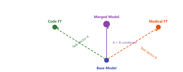
Model merging exploits a remarkable property of neural network loss landscapes: models fine-tuned from the same base occupy a connected region of parameter space where linear interpolations between them tend to perform well. When two models are fine-tuned from the same pretrained checkpoint, their weight differences from the base represent "task vectors" in parameter space. These task vectors can be combined arithmetically because the underlying loss landscape in the neighborhood of the pretrained model is approximately convex.
The key constraint is that all models being merged must share the same architecture and originate from the same base pretrained checkpoint. You cannot merge a Llama model with a Mistral model (for an overview of these model families, see Chapter 7), or even two Llama models fine-tuned from different pretrained versions. The common ancestry is what ensures the weight spaces are compatible. visualizes these task vectors in parameter space.
When merging models with MergeKit, always evaluate the merged model on benchmarks from all constituent tasks, not just the one you care about most. A common failure mode is that merging improves your target task while catastrophically degrading another. The TIES and DARE methods are specifically designed to minimize this interference by resolving sign conflicts and pruning redundant updates before merging.
Think of model merging as mixing cocktails. Each fine-tuned model is a single spirit with a distinct flavor profile (one excels at code, another at creative writing, a third at math). Weight averaging is the simplest mix: equal parts of each. SLERP and TIES are more sophisticated bartending techniques that blend flavors along smooth curves or resolve conflicting ingredients. The result can be a balanced cocktail that inherits the best of each spirit, though poor mixing ratios can produce something undrinkable.
Why does model merging work at all? This is one of the most surprising results in recent LLM research. The intuition relies on the concept of linear mode connectivity: models fine-tuned from the same base checkpoint tend to occupy the same low-loss basin in the parameter space. Because they share the same initialization, the paths from the base model to each fine-tuned variant do not cross high-loss barriers. Averaging (or otherwise combining) their weights produces a point that also lies within this shared basin, inheriting capabilities from both. This explains why merging fails for models trained from different random initializations: they occupy entirely separate loss basins with no linear path between them. The practical consequence is that model merging is only reliable when all constituent models descend from the same base checkpoint.
Model merging gives you multi-task capability without multi-task training data. If you have one LoRA adapter fine-tuned for code generation and another for medical Q&A, merging them can produce a model competent at both tasks, without ever creating a dataset that mixes code and medical examples. This is uniquely valuable in practice because collecting balanced multi-task training data is one of the hardest parts of fine-tuning. Merging bypasses this entirely by combining independently trained specialists.
Model merging only works when all models share the same base architecture and were fine-tuned from the same pretrained checkpoint. Merging a Llama-3 fine-tune with a Mistral fine-tune will produce garbage, not a model that combines both capabilities. The reason is that merging relies on parameter-space proximity: models fine-tuned from the same starting point differ only slightly, and interpolating between them stays in a "good" region of the loss landscape. Models with different architectures (or even the same architecture trained from scratch separately) occupy entirely different regions. Always verify that all models you intend to merge share the exact same base model before proceeding.
17.7.2 Merging Methods
Linear mode connectivity explains why merging works at all; it does not tell us which arithmetic to use. Four families of methods (linear averaging, SLERP, TIES-Merging, and DARE) trade simplicity for sophistication, each fixing a failure mode of the last. We work up the ladder, starting with the simplest weighted average and noting where it breaks down.
17.7.2.1 Linear (Weighted Average)
The simplest merging method computes a weighted average of model weights. Given models A and B with weights $W_{A}$ and $W_{B}$, the merged model has weights:
The mixing coefficient α controls the balance between models. Setting α = 0.5 gives equal weight to both. Linear merging is fast and simple, but it can produce mediocre results when the models have very different weight distributions because opposing parameter changes can cancel each other out.
A tiny numeric example clarifies the effect. Consider a single parameter from two fine-tuned models:
# Linear merge of a single weight with different alpha values
w_a, w_b = 1.4, 0.6 # same parameter in models A and B
for alpha in [0.3, 0.5, 0.7]:
    w_merged = alpha * w_a + (1 - alpha) * w_b
    print(f"alpha={alpha:.1f} -> W_merged = {alpha}*{w_a} + {1-alpha}*{w_b} = {w_merged:.2f}")
    # alpha=0.3 -> W_merged = 0.84 (closer to model B)
    # alpha=0.5 -> W_merged = 1.00 (midpoint)
# alpha=0.7 -> W_merged = 1.16 (closer to model A)alpha=0.3 -> W_merged = 0.3*1.4 + 0.7*0.6 = 0.84 alpha=0.5 -> W_merged = 0.5*1.4 + 0.5*0.6 = 1.00 alpha=0.7 -> W_merged = 0.7*1.4 + 0.3*0.6 = 1.16
Uniform Soup, Grid-Searched Soup, and Greedy Soup
The Model Soup family (Wortsman et al., 2022) is the practical packaging of linear averaging. Uniform soup averages all candidate checkpoints with equal weights and is the cheapest baseline. Grid-searched soup sweeps a small set of mixing coefficients per checkpoint on a held-out validation set; it works for two or three checkpoints but becomes combinatorially expensive beyond that. Greedy soup is the standard fix: sort the checkpoints by individual validation score, start with the best one as the running average, and iteratively try adding the next-best checkpoint to the soup only if doing so improves validation accuracy. Reject any checkpoint whose addition hurts. The procedure is one validation pass per candidate, runs in linear time, and consistently outperforms uniform soup when the candidate pool contains low-quality outliers (as it typically does after a hyperparameter sweep).
# Greedy soup pseudo-code
candidates = sorted(checkpoints, key=val_score, reverse=True)
soup = [candidates[0]]
best = val_score(candidates[0])
for ckpt in candidates[1:]:
    trial = average_weights(soup + [ckpt])
    if val_score(trial) > best:
        soup.append(ckpt)
        best = val_score(trial)
final = average_weights(soup)17.7.2.2 SLERP (Spherical Linear Interpolation)
SLERP treats weight vectors as points on a high-dimensional sphere and interpolates along the geodesic (shortest path on the sphere surface) rather than in a straight line through the interior. This preserves the magnitude of weight vectors better than linear interpolation, which tends to shrink weights toward zero when the models diverge.
SLERP is applied layer by layer (or parameter by parameter) and produces consistently better results than linear averaging. It is the recommended default for merging two models.
SLERP can only merge exactly two models at a time. For merging three or more models, you must either chain multiple SLERP operations (merge A+B, then merge result+C) or use a method that natively supports multiple inputs like Linear averaging or TIES. The order of chained SLERP merges can affect the result, so experiment with different orderings.
Who: Open-source model developer contributing to the Hugging Face community
Situation: The developer had three separately fine-tuned LoRA adapters on Mistral 7B: one for creative writing, one for code generation, and one for factual Q&A.
Problem: Serving three separate adapters required either runtime adapter switching (adding latency) or running three model instances (tripling GPU cost).
Dilemma: Linear averaging of the three adapters degraded performance on all tasks because the code adapter and creative writing adapter pushed parameters in opposite directions for shared layers.
Decision: They used TIES-Merging with density 0.5 to resolve parameter conflicts, trimming low-magnitude deltas and electing the majority sign direction before averaging.
How: Using the mergekit library, they defined a YAML config specifying TIES as the merge method, set density to 0.5, and assigned equal weight to all three models. The merge completed in 4 minutes on CPU.
Result: The merged model retained 92% of each specialist's benchmark score on its domain, compared to only 78% with naive linear averaging. A single model served all three tasks with no adapter switching overhead.
Lesson: When merging models with conflicting parameter updates, TIES resolves sign conflicts that destroy performance under simple averaging; always try TIES before concluding that merging does not work for your use case.
Model merging combines multiple fine-tuned models into one without any additional training. It is like mixing paint colors: if blue is good at code and red is good at creative writing, maybe purple can do both. Surprisingly, this metaphor holds up better than you would expect.
17.7.2.3 TIES (TRIM, Elect Sign, merge)
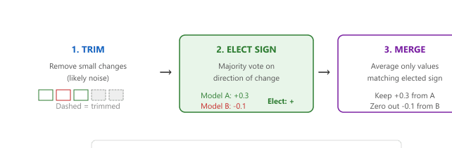
TIES-Merging (2023) addresses the interference problem that plagues simple averaging. When two fine-tuned models modify the same parameter in opposite directions, averaging cancels out both changes. TIES handles this through three steps:
A concrete interference case: pick a single parameter at layer 10. The code fine-tune pushed it from 0.50 (base) to 0.85 (delta +0.35). The creative-writing fine-tune pushed the same parameter from 0.50 to 0.15 (delta -0.35). Naive averaging gives back (0.85 + 0.15) / 2 = 0.50, exactly the base value: both fine-tunes' knowledge cancels out. TIES looks at the two deltas (+0.35 and -0.35), trims any tiny ones (these are large, so both survive), votes on the sign (here it is a tie, but with three models the majority wins), and merges only deltas matching the elected sign. If "+" wins, the resulting parameter becomes 0.50 + 0.35 = 0.85 (just the code knowledge); the conflicting -0.35 is zeroed rather than averaged in. The result preserves more useful capability than the averaged 0.50 ever could.
- TRIM: Remove small-magnitude changes (below a threshold) that are likely noise rather than meaningful task knowledge.
- Elect Sign: For each parameter, take a majority vote across models on the sign of the change. Parameters where models disagree on direction are resolved by the majority.
- Merge: Average only the values that agree with the elected sign, zeroing out conflicting contributions.
Formally, given a base model $\theta_0$ and $N$ task-specific fine-tunes $\theta_1, \dots, \theta_N$, let $\tau_i = \theta_i - \theta_0$ be the task vector (delta) for model $i$, with $\tau_i^{(j)}$ the $j$-th parameter. The three TIES steps are:
$$\begin{aligned}\hat{\tau}_i^{(j)} &= \tau_i^{(j)} \cdot \mathbb{1}\!\big[|\tau_i^{(j)}| \ge q_{1-k}\big(|\tau_i|\big)\big] &&\text{(TRIM: keep top-}k\%)\\[2pt] s^{(j)} &= \operatorname{sign}\!\Big(\sum_{i=1}^{N} \hat{\tau}_i^{(j)}\Big) &&\text{(ELECT SIGN: aggregate vote)}\\[2pt] \tau_{\text{TIES}}^{(j)} &= \frac{1}{|\mathcal{A}^{(j)}|}\sum_{i \in \mathcal{A}^{(j)}} \hat{\tau}_i^{(j)}, \quad \mathcal{A}^{(j)} = \{i : \operatorname{sign}(\hat{\tau}_i^{(j)}) = s^{(j)}\} &&\text{(MERGE aligned only)}\\[2pt] \theta_{\text{merged}} &= \theta_0 + \lambda \cdot \tau_{\text{TIES}} &&\text{(rescaled add-back)}\end{aligned}$$
where $q_{1-k}(\cdot)$ is the $(1-k)$-quantile of the absolute deltas (the density parameter in MergeKit), $\mathbb{1}[\cdot]$ is the indicator function, $\mathcal{A}^{(j)}$ is the set of models that survived TRIM and whose sign matches the elected direction, and $\lambda$ is a global merge scale (typically 1.0). The crucial line is the third one: averaging is restricted to $\mathcal{A}^{(j)}$ rather than over all $N$ models, which is exactly what prevents the +0.35 / -0.35 cancellation in the concrete case above. Figure 17.7.2 walks through these three TIES steps visually.
17.7.2.4 DARE (Drop And REscale)
DARE (2024) takes a different approach to reducing interference: it randomly drops a large fraction (typically 90-99%) of the delta parameters before merging, then rescales the remaining parameters to compensate. The intuition is that fine-tuning changes are highly redundant, and a small random subset of changes captures the essential task knowledge. By keeping only a sparse set of changes from each model, the probability of destructive interference is dramatically reduced.
DARE can be combined with other merging methods (DARE+TIES is a popular combination) and tends to work especially well when merging many models or when the models have been fine-tuned for very different tasks.
17.7.2.5 Model Stock
Model Stock (2024) draws on ideas from portfolio theory in finance. Instead of merging all models uniformly, it selects an optimal subset and weighting based on the geometric properties of the models in weight space. It computes the distances between models and the base, then assigns weights that maximize diversity while minimizing deviation from the base. This produces more robust merges, particularly when some of the input models are lower quality or overfitted.
17.7.2.6 Frankenmerging (Flow-Space Layer Stacking)
Every method above lives in parameter space: it averages or combines weight tensors of two architectures with identical shapes. Frankenmerging lives in flow space: instead of mixing weights at the same depth, it physically stacks layers from different donor models into a single new architecture. The output network can be deeper than any donor (for example, 60 transformer blocks stitched together from two 32-block donors with overlap) or rearranged (alternating blocks from donor A and donor B), giving the merged model a literally different forward pass. MergeKit calls this the passthrough merge method, and the technique is occasionally followed by a short fine-tuning pass on a small target dataset (the concat-then-finetune recipe) to smooth the seams between donor regions.
# Frankenmerge YAML: stack layers 0-23 from donor A on top of layers 8-31 from donor B
# producing a 48-block model out of two 32-block donors
merge_method: passthrough
dtype: bfloat16
slices:
  - sources:
      - model: donor-A-7b
        layer_range: [0, 24]
  - sources:
      - model: donor-B-7b
layer_range: [8, 32]Frankenmerging produced several viral open-source models in 2024 (Goliath-120B is a stack of two Llama 2 70B models; SOLAR-10.7B is a depth-up-scaled Mistral). The method is constrained to the same hidden dimension and attention configuration across donors (otherwise the residual stream shapes do not match), and its quality is highly variable: the merged model can outperform either donor on some tasks while regressing badly on others, and the post-merge finetune is often the dominant source of any quality gain.
The marketing around model merging often promises capability composition for free. The empirical record is more sober. Three regimes consistently work in practice:
- Checkpoint averaging within one training run (the original Model Soup setting): averaging several late-stage checkpoints of the same fine-tune reduces variance and is essentially free quality. This is by far the most reliable use case.
- Closely-related LoRA adapters on top of the same base, where SLERP or weighted-average soup blends two style adapters into a usable hybrid for personalization or A/B testing.
- Frankenmerging followed by a short SFT pass, where the fine-tune (not the merge) does most of the heavy lifting.
Three regimes consistently disappoint:
- Cross-task capability stacking ("merge a code model and a math model, get a code+math model"). The naive expectation rarely holds. TIES and DARE help but typically leave the merged model 5 to 15 percent below either specialist on its own benchmark.
- Different base models. The base-model warning in Section 17.7.1 is absolute: merging across base architectures produces noise.
- Recovering data you do not have. Merging cannot create knowledge that is in neither input model. If two donors both fail on a benchmark, the merged model will too.
The honest summary is that model merging has not delivered on the early "free composition" hype. It survives, productively, in two niches: checkpoint averaging for variance reduction (always worth running), and hobbyist Frankenmodels that combine layers across donors and then fine-tune. Reach for full fine-tuning or LoRA when capability composition genuinely matters.
17.7.3 Merging Method Comparison
provides an at-a-glance comparison of the merging methods covered above. The table below adds quantitative detail on each method's capabilities and trade-offs.
| Method | Models | Handles Interference | Complexity | Best For |
|---|---|---|---|---|
| Linear | 2+ | No | Very Low | Quick baseline, similar models |
| SLERP | 2 only | Partially | Low | Default for two-model merges |
| TIES | 2+ | Yes (sign election) | Medium | Merging 3+ diverse models |
| DARE | 2+ | Yes (sparsification) | Medium | Many models, high diversity |
| DARE+TIES | 2+ | Yes (both) | Medium | Best overall quality |
| Model Stock | 2+ | Yes (selection) | High | Quality-sensitive merges |
| Frankenmerge (passthrough) | 2+ (same hidden dim) | N/A (flow-space) | Low + post-finetune | Depth upscaling, hobbyist hybrids |
17.7.4 Task Arithmetic
Task arithmetic provides the theoretical framework for understanding model merging. A "task vector" is defined as the element-wise difference between a fine-tuned model and its pretrained base: τ = $W_{ft}$ - $W_{base}$. Task arithmetic shows that these vectors can be manipulated algebraically:
- Addition: $W_{base}$ + τA + τB creates a model with both capabilities
- Negation: $W_{base}$ - τA removes capability A (useful for unlearning)
- Scaling: $W_{base}$ + λτA controls the strength of adaptation
Code Fragment 17.7.3a demonstrates this approach.
# Implement model merging by interpolating weight tensors
# Linear interpolation (LERP/SLERP) blends capabilities from multiple models
import torch
from transformers import AutoModelForCausalLM
def compute_task_vector(base_model_id, finetuned_model_id):
    """Compute task vector: delta = finetuned - base."""
    # Load pretrained causal LM (decoder-only architecture)
    base = AutoModelForCausalLM.from_pretrained(base_model_id)
    finetuned = AutoModelForCausalLM.from_pretrained(finetuned_model_id)
    task_vector = {}
    for name in base.state_dict():
        task_vector[name] = (
            finetuned.state_dict()[name].float()
            - base.state_dict()[name].float()
            )
        return task_vector
    def apply_task_vectors(base_model_id, task_vectors, scaling_factors):
        """Apply scaled task vectors to base model."""
        model = AutoModelForCausalLM.from_pretrained(base_model_id)
        state_dict = model.state_dict()
        for tv, scale in zip(task_vectors, scaling_factors):
            for name in state_dict:
                state_dict[name] = state_dict[name].float() + scale * tv[name]
                model.load_state_dict(state_dict)
                return model
                # Example: combine code and medical capabilities
                code_tv = compute_task_vector("base-model", "code-finetuned")
                medical_tv = compute_task_vector("base-model", "medical-finetuned")
                merged = apply_task_vectors(
                    "base-model",
                    [code_tv, medical_tv],
                    [0.7, 0.5], # Scaling factors per task
                    )
Merge complete. Test with: transformers AutoModelForCausalLM.from_pretrained('./merged-output')
Code Fragment 17.7.4a demonstrates model merging with a TIES configuration file.
# TIES merge configuration (merge_ties.yml)
models:
 - model: models/code-llama-7b
 parameters:
 density: 0.5 # Keep top 50% of changes
 weight: 1.0
 - model: models/medical-llama-7b
 parameters:
 density: 0.5
 weight: 0.8
 - model: models/math-llama-7b
 parameters:
 density: 0.5
 weight: 0.6

merge_method: ties
base_model: meta-llama/Llama-3-8B
parameters:
 normalize: true
dtype: bfloat16normalize flag ensures merged weights maintain proper scale.Run the merge from the command line or use the MergeKit Python API for programmatic control. Code Fragment 17.7.4b shows both approaches.
# pip install mergekit
# Option 1: CLI (most common)
# mergekit-yaml merge_ties.yml ./merged-output --cuda --copy-tokenizer
# Option 2: Python API for programmatic merging
from mergekit.config import MergeConfiguration
from mergekit.merge import MergeOptions, run_merge
config = MergeConfiguration.from_yaml("merge_ties.yml")
run_merge(
    config,
    out_path="./merged-output",
    options=MergeOptions(
    cuda=True,
    copy_tokenizer=True,
    lazy_unpickle=True, # lower RAM usage
    ),
)
print("Merge complete. Test with: transformers AutoModelForCausalLM.from_pretrained('./merged-output')")Model merging requires enough system memory (RAM, not GPU VRAM) to hold all models simultaneously. Merging three 7B models in BF16 requires roughly 42 GB of RAM. Use the --lazy-unpickle flag in MergeKit to reduce memory usage by loading models incrementally. For very large models, consider merging on a cloud instance with sufficient RAM rather than on a local machine.
17.7.5 Evolutionary Model Merging
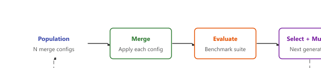
Evolutionary model merging (Sakana AI, 2024) automates the search for optimal merge configurations using evolutionary algorithms. Instead of manually selecting merge methods, weights, and layer-specific parameters, an evolutionary optimizer explores the space of possible merges and evaluates each candidate against a benchmark suite. This approach has produced merged models that significantly outperform manually configured merges.
The search space includes merge method selection, per-layer interpolation weights, density parameters (for TIES/DARE), and even layer permutations. The evolutionary algorithm (typically CMA-ES or NSGA-II) optimizes these parameters against multiple objectives: performance on target benchmarks, retention of base model capabilities, and overall coherence. The diagram below depicts this optimization loop.
Set temperature to 2.0 to 4.0 when computing the teacher's soft labels. Higher temperatures reveal more of the teacher's uncertainty and inter-class relationships, giving the student richer learning signals than hard labels or low-temperature outputs.
Model merging has moved beyond simple weight averaging with methods like TIES-Merging (which resolves sign conflicts between parameter deltas) and DARE (which randomly prunes delta parameters before merging). The evolutionary model merging approach by Sakana AI uses optimization algorithms to search over merging configurations, discovering non-obvious combinations that outperform expert-designed blends.
The key open problem is predicting merge quality before performing the merge, since current approaches require expensive post-merge evaluation to determine whether a combination was successful.
- Model merging combines specialized models into multi-skilled models with zero additional training, requiring only system RAM (not GPU VRAM).
- All models must share the same base architecture and pretrained checkpoint for merging to produce meaningful results.
- SLERP is the best default for two-model merges, preserving weight magnitudes through spherical interpolation rather than linear averaging.
- TIES and DARE handle interference when merging three or more models, using sign election and sparsification to prevent conflicting changes from canceling out.
- Task arithmetic provides the theoretical foundation: task vectors (fine-tuning deltas) can be added, subtracted, and scaled to compose and decompose model capabilities.
- Model soups average checkpoints from the same training process to improve robustness and generalization for a single task.
- MergeKit is the standard tool for practical model merging, supporting all major algorithms through YAML configuration files.
- Evolutionary merging automates the search for optimal merge configurations, often outperforming manually tuned merges.
Show Answer
Show Answer
Show Answer
Show Answer
Show Answer
Exercises
Explain the concept of task arithmetic in model merging. What does it mean to compute a 'task vector', and how can you add or subtract task vectors?
Answer Sketch
A task vector is the difference between a fine-tuned model's weights and the base model's weights: task_vector = W_finetuned - W_base. This vector captures what the fine-tuning learned. You can add task vectors to give the base model multiple skills: W_merged = W_base + task_vector_code + task_vector_medical. You can subtract to remove capabilities: W_detoxified = W_base + task_vector - toxic_vector. This treats model capabilities as compositional vectors in weight space.
Compare linear interpolation and SLERP (Spherical Linear Interpolation) for merging two models. When does SLERP produce better results?
Answer Sketch
Linear: W = (1-t)*W_A + t*W_B. Simple but can reduce the magnitude of weight vectors, potentially degrading quality. SLERP: interpolates along the great circle on the unit hypersphere, preserving the magnitude of weight vectors. SLERP produces better results when the two models have similar magnitudes but different directions, which is common for models fine-tuned from the same base. For very similar models, the difference is minimal.
Write a MergeKit YAML configuration that merges a code-specialized model and a math-specialized model using the TIES method with density 0.5.
Answer Sketch
Config: merge_method: ties; base_model: meta-llama/Llama-3-8B; models: [{model: code-llama-8b, parameters: {density: 0.5, weight: 1.0}}, {model: math-llama-8b, parameters: {density: 0.5, weight: 1.0}}]; parameters: {normalize: true}; dtype: float16. Run: mergekit-yaml config.yaml output_dir/. TIES resolves sign conflicts between task vectors by keeping only the top 50% (density) of parameters and resolving sign disagreements by majority vote.
Explain the DARE (Drop And REscale) merging method. How does randomly dropping delta parameters before merging improve the result compared to naive averaging?
Answer Sketch
DARE randomly sets a fraction (1 minus p) of each task vector's parameters to zero, then rescales the remaining parameters by 1/p to preserve the expected magnitude. This works because most parameters in a task vector are noise; only a small fraction carry the task-specific signal. Dropping noise reduces interference between task vectors during merging, allowing more models to be merged simultaneously without quality degradation. DARE enables merging 5+ models where naive averaging fails.
After merging a code model and a medical model, write an evaluation script that tests the merged model on both code generation and medical QA benchmarks, plus a general knowledge benchmark to check for degradation.
Answer Sketch
Run three evaluation suites: (1) Code: HumanEval or MBPP, measure pass@1. (2) Medical: MedQA or PubMedQA, measure accuracy. (3) General: MMLU or HellaSwag, measure accuracy. Compare against: the base model, the code-only fine-tune, and the medical-only fine-tune. The merged model should approach the specialist accuracy on each domain while retaining general capability above the base model. Report results in a comparison table with confidence intervals.
What Comes Next
In the next section, Section 17.8: Continual Learning and Domain Adaptation, we address continual learning and domain adaptation, keeping models current as data distributions shift over time. Model merging approaches also relate to the LoRA adapter concepts in Section 17.1, since adapters can themselves be merged.