"An image is worth 16x16 words."Dosovitskiy et al., the original ViT paper, 2020
Modern Vision-Language Models are stitched together from two halves: a vision encoder that turns pixels into a sequence of vectors, and a language model that consumes those vectors as if they were token embeddings. The dominant vision encoder, in every frontier VLM as of 2026, is some variant of the Vision Transformer (ViT). This section explains how ViT turns an image into a token sequence (patch embedding, position encoding, class token), traces the lineage from ViT-B/16 through DINOv2, SigLIP-ViT, and the InternViT-6B family, and lays the foundation for the contrastive and generative VLMs that follow.
Prerequisites
This section assumes the transformer mechanics from Section 3.1, the tokenization and embedding intuition from Section 1.6, and the basic CNN-versus-attention contrast from Section 0.5.
Before diving into ViT specifics, it helps to have a four-bucket taxonomy that places every later model (CLIP, BLIP, DINO, SAM, ViT variants) onto the same shelf. Pretrained vision models fall into four families, each defined by what the model produces and how downstream code consumes it.
| Family | Output | Defining feature | Canonical examples |
|---|---|---|---|
| Task-specific | Class labels, masks, or boxes | The task is baked into the model; downstream code consumes the prediction directly. | Faster R-CNN (detection), DeepLab (segmentation), ViT-ImageNet classifier |
| Representation | An embedding vector (or per-patch vectors) | Task-agnostic backbone; downstream head chooses what to do with the embedding. | ResNet, ViT, DINO, DINOv2, DeiT |
| Multimodal | An embedding aligned with text (or another modality) | The space is shared across modalities, enabling cross-modal comparison. | CLIP, SigLIP, BLIP-2, LLaVA |
| Generative | A whole new image (pixels) | The output is an image, not a representation; conditioned on a prompt, mask, or reference image. | VAE, GAN, latent diffusion, flow-based models |
Chapter 22 lives mostly in the second and third buckets. ViT, DINO, DeiT, and Swin (this section) are representation backbones. CLIP, SigLIP, BLIP-2, LLaVA, and the frontier VLMs in later sections add text alignment, moving into the multimodal bucket. Keeping this shelf in mind makes it easier to know what each model is actually for when later sections introduce a new acronym.
22.1.1 From Pixels to Tokens: The Patch Embedding
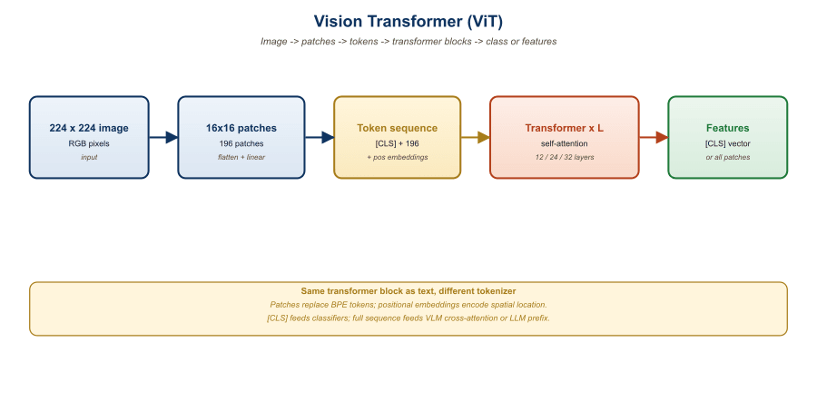
The defining move of ViT (Dosovitskiy et al., Google, 2020) was to abandon convolutions entirely and treat an image as a sequence of small fixed-size patches. For a 224x224 RGB image with a patch size of 16x16, the image is partitioned into 14x14 = 196 non-overlapping patches. Each patch is flattened to a 16x16x3 = 768-dimensional vector and linearly projected to the model's hidden dimension (typically 768 for ViT-Base, 1024 for ViT-Large, 1280 for ViT-Huge). The resulting sequence of 196 patch embeddings is then processed by a standard transformer encoder, exactly the same architecture used in BERT for text.
This reframing has two consequences. The first is computational: ViT inherits the quadratic complexity of self-attention in the sequence length. A 224x224 image with 16x16 patches has 196 tokens, which is manageable, but a 1024x1024 image with the same patch size yields 4096 tokens (16x the FLOPs and 256x the memory). This drives much of the design space for VLMs that need to handle high-resolution inputs, as we will see in Section 22.3.
The second consequence is inductive bias. CNNs build in translation equivariance and locality through their architecture; ViTs do not. A patch in the top-left corner has no architectural reason to "know" that it is adjacent to its neighbor. Position encodings (described below) compensate by injecting spatial information through learned embeddings. The practical implication is that ViTs need more training data than equivalently-sized CNNs to reach competitive accuracy, but once trained at scale, they exceed CNN performance on most visual benchmarks.
Concretely, think of patch embedding as photocopying a photograph onto sticky notes. You print the photo onto a 14x14 grid of sticky notes, each capturing a small 16x16 pixel square. The transformer then reads these sticky notes one by one (in arbitrary order) and decides for itself which notes are adjacent or related. Position encodings are the page-number stamps you add to each note so the reader can reconstruct the original layout; without them, the model sees a shuffled pile of patches with no spatial structure.
22.1.2 Position Encoding and the Class Token
Two additional ingredients complete the basic ViT input. The first is the position encoding: a learned embedding for each of the 196 patch positions, added element-wise to the patch embeddings. The original ViT used 1D learned position embeddings (treating the 14x14 grid as a flattened sequence), which is sufficient for fixed input resolutions. Subsequent models adopted 2D sinusoidal or 2D learned position embeddings for better generalization across resolutions, and the most recent generation (DINOv2, EVA-CLIP) uses 2D rotary position embeddings (2D-RoPE) for arbitrary input sizes.
The second ingredient is the [CLS] (class) token: a learned vector prepended to the sequence of patch embeddings. After 12 (or 24, or 32) layers of self-attention, the final hidden state at the [CLS] position serves as a global image representation suitable for classification or contrastive matching. This is the direct visual analog of BERT's [CLS] token for text. For dense prediction tasks (segmentation, detection), per-patch embeddings are used instead.
There are two natural ways to turn the 197-token ViT output into a single per-image vector. The first is to read off the [CLS] token, which is what the original ViT classifier head consumes and what CLIP uses for its image embedding. The second is to mean-pool the 196 patch tokens, ignoring [CLS] altogether. These two embeddings live in the same dimension but they are not the same vector and they do not have the same downstream properties. [CLS] was trained (via the supervised or contrastive head) to summarize what the image is about, so it captures category-level semantics cleanly. Mean-pooled patch features instead carry a more uniform mixture of every spatial region, which makes them better for tasks that care about every part of the image (texture analysis, retrieval against scene-rich queries). DINOv2 deliberately uses both signals at different stages, and Hugging Face AutoModel exposes both via outputs.pooler_output (CLS-derived) and outputs.last_hidden_state[:, 1:].mean(dim=1) (mean pool). If a downstream classifier underperforms, switching pooling strategy is often the cheapest experiment to run.
[CLS] token is prepended. The 197-token sequence is processed by a standard transformer encoder.22.1.3 Running ViT Inference
The Hugging Face transformers library ships ViT support through the ViTModel class for feature extraction and ViTForImageClassification for pretrained classifier heads. The minimum viable call demonstrates both the input preparation and the structure of the output.
Before running it, the patch tokenization is worth pinning down. A ViT-Base/16 model splits a 224x224 RGB image into a 14x14 grid of 16x16 patches, flattens each patch into a 768-dim vector, and prepends a learned $\texttt{[CLS]}$ token, giving the well-known 197-token sequence length:
Each patch $x_p \in \mathbb{R}^{P \cdot P \cdot 3}$ is mapped through a single linear projection $E \in \mathbb{R}^{(P^2 \cdot 3) \times D}$, summed with a learned positional embedding, and fed through the standard transformer encoder. The 197 output tokens in the code below are exactly the $\texttt{[CLS]}$ plus the 196 patches.
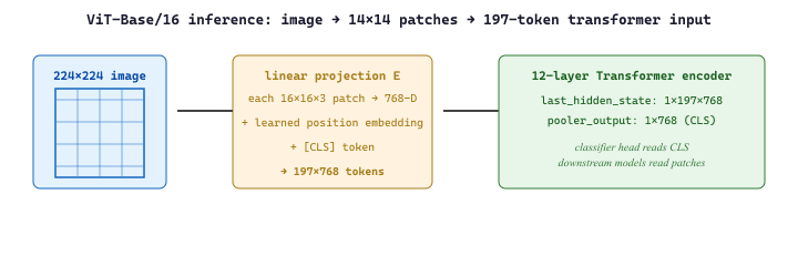
[CLS] token is prepended, and the resulting 197-token sequence runs through a standard transformer encoder. The last_hidden_state and pooler_output from the code block below correspond exactly to the two outputs on the right.LLaVA-1.5 uses CLIP ViT-L/14 at input resolution 336x336 instead of 224x224 and patch size 14 instead of 16. The patch grid is therefore (336/14)x(336/14) = 24x24 = 576 patches, plus the [CLS] token, giving N=577 transformer tokens per image. Each token is 1024-dim (ViT-L's hidden size). The output tensor shape that LLaVA's projector consumes is exactly (batch, 576, 1024) after dropping the [CLS]: 576 visual tokens that get mapped into the LLM's embedding space. This is the source of the "576 visual tokens" number in Section 22.7.
from transformers import ViTImageProcessor, ViTModel
from PIL import Image
import torch

# Load ViT-Base pretrained on ImageNet-21k then fine-tuned on ImageNet-1k
processor = ViTImageProcessor.from_pretrained("google/vit-base-patch16-224")
model = ViTModel.from_pretrained("google/vit-base-patch16-224").eval()

image = Image.open("cat.jpg").convert("RGB")
inputs = processor(image, return_tensors="pt")
print(f"Input pixel tensor shape: {inputs.pixel_values.shape}")

with torch.inference_mode():
    outputs = model(**inputs)

# Two key outputs:
#   last_hidden_state: [batch, 197, 768] - per-token representations
#   pooler_output:     [batch, 768]      - CLS token after Tanh projection
print(f"Token-level features: {outputs.last_hidden_state.shape}")
print(f"Global image feature: {outputs.pooler_output.shape}")

# The 197 tokens decompose as: 1 CLS + 196 patches (14x14 grid)
cls_feature = outputs.last_hidden_state[:, 0, :]
patch_features = outputs.last_hidden_state[:, 1:, :].reshape(1, 14, 14, 768)
print(f"Reshaped patch grid: {patch_features.shape}")The same ViTModel backbone wraps into a one-shot training loop for any custom label vocabulary. The Hugging Face Trainer takes care of evaluation, checkpointing, and mixed precision; the only bespoke piece is the label map.
from transformers import (
    ViTForImageClassification, ViTImageProcessor,
    Trainer, TrainingArguments,
)
from datasets import load_dataset

ds = load_dataset("food101", split={"train": "train[:5000]", "val": "validation[:1000]"})
labels = ds["train"].features["label"].names
id2label = {i: l for i, l in enumerate(labels)}
label2id = {l: i for i, l in id2label.items()}

processor = ViTImageProcessor.from_pretrained("google/vit-base-patch16-224-in21k")
model = ViTForImageClassification.from_pretrained(
    "google/vit-base-patch16-224-in21k",
    num_labels=len(labels),
    id2label=id2label, label2id=label2id,
    ignore_mismatched_sizes=True,   # swap in the new classifier head
)

def transform(batch):
    px = processor([img.convert("RGB") for img in batch["image"]], return_tensors="pt")
    return {"pixel_values": px["pixel_values"], "labels": batch["label"]}

ds = ds.with_transform(transform)
args = TrainingArguments(
    output_dir="vit-food101",
    per_device_train_batch_size=32, per_device_eval_batch_size=32,
    num_train_epochs=3, learning_rate=2e-5,
    eval_strategy="epoch", save_strategy="epoch",
    fp16=True, report_to="none",
)
Trainer(model=model, args=args, train_dataset=ds["train"], eval_dataset=ds["val"]).train()
Code Fragment 22.1.2a: Fine-tuning ViT-Base on a custom 101-class food dataset. ignore_mismatched_sizes=True lets the Trainer drop the original ImageNet head and initialize a new classifier matched to the user vocabulary. A 5k-image subset trains to ~85% top-1 in three epochs on a single RTX 4090.
22.1.4 The ViT Zoo: Resolution and Patch Size Tradeoffs
Production ViTs come in many sizes. The naming convention is ViT-{S, B, L, H, G}/{8, 14, 16, 32} where the first letter is the model size and the number is the patch size in pixels. ViT-B/16 means base-size (86M parameters) with 16x16 patches; ViT-L/14 means large-size (303M parameters) with 14x14 patches. Smaller patches mean more tokens per image, more FLOPs, and typically better accuracy on dense tasks.
The other axis is input resolution. The original ViT used 224x224, but modern VLMs span a wide range:
- 336x336 (the CLIP variant), the most common production default.
- 384x384 (TrOCR), useful for OCR-heavy workloads.
- 448x448 (Qwen-VL), better for dense charts and tables.
- Arbitrary "any-resolution" inputs via interpolation of the position embeddings, used by the latest open VLMs.
Higher resolution improves performance on tasks requiring small-detail recognition (small text in documents, individual fingers in human poses) at quadratic compute cost.
| Variant | Params | Patch Size | Resolution | Tokens | FLOPs (forward) |
|---|---|---|---|---|---|
| ViT-S/16 | 22M | 16 | 224 | 197 | 4.6 GFLOPs |
| ViT-B/16 | 86M | 16 | 224 | 197 | 17.6 GFLOPs |
| ViT-L/14 | 303M | 14 | 224 | 257 | 81 GFLOPs |
| ViT-L/14@336 | 303M | 14 | 336 | 577 | 190 GFLOPs |
| ViT-H/14 | 632M | 14 | 224 | 257 | 167 GFLOPs |
| ViT-G/14 | 1.8B | 14 | 224 | 257 | 480 GFLOPs |
| InternViT-6B | 5.9B | 14 | 448 | 1025 | 5.7 TFLOPs |
The most common vision encoder in production VLMs as of 2026 is ViT-L/14 at 336x336 (the version used by CLIP, LLaVA, BLIP-3, and others). The choice represents a sweet spot: 577 tokens per image is enough for dense scenes, 303M parameters fit comfortably alongside a 7B-70B language model, and the CLIP pretraining provides strong zero-shot transfer. Larger encoders (ViT-H, ViT-G) give marginal gains; smaller encoders (ViT-B) cause noticeable accuracy losses on text-in-image tasks.
22.1.5 Pretraining Objectives: Supervised vs. Self-Supervised
The pretraining recipe determines what the encoder learns to represent. Four main objectives have shaped the modern ViT landscape.
The first is supervised classification on ImageNet-21k or JFT-300M. The original ViT was pretrained this way, predicting 21,000 or 18,000 class labels respectively. The learned features are excellent for classification transfer but suboptimal for tasks needing fine-grained semantic structure.
The second is masked image modeling (MIM), inspired by masked language modeling in BERT. MAE (He et al., 2021) and BEiT (Bao et al., 2021) randomly mask 75% of input patches and train the model to reconstruct the missing pixels (MAE) or patch tokens from a learned codebook (BEiT). MIM produces strong features for dense prediction (segmentation, detection) and is the dominant pretraining for image-only models, but does not directly produce text-aligned representations.
The third is contrastive image-text learning. CLIP (Radford et al., 2021) and SigLIP (Zhai et al., 2023) train the ViT to produce image embeddings that match corresponding text embeddings in a shared space. This is the dominant pretraining for VLM vision encoders because the resulting features are explicitly language-aligned. We explore CLIP and SigLIP in depth in Section 22.2.
The fourth is self-supervised learning via image-only objectives that produce semantically meaningful features without text. DINO (Caron et al., 2021) and DINOv2 (Oquab et al., 2023) use a teacher-student setup where the model learns to produce consistent representations across augmentations. DINOv2's features are remarkable: they cluster semantic concepts (animals, vehicles, faces) without ever seeing class labels and serve as drop-in replacements for CLIP encoders in some VLMs (notably Idefics-2).
DeiT: The Distillation-Token Bridge to ImageNet-1K
The original ViT paper made an uncomfortable confession: ViTs only outperform CNNs when pretrained on JFT-300M (Google's 300-million-image internal dataset). On the public ImageNet-1K (1.3M images), a plain ViT trails a same-sized ResNet. For two years that gating fact kept ViTs out of academic labs that could not access JFT.
DeiT (Touvron et al., Facebook AI, 2021) fixed the problem with a single architectural addition: the distillation token. Alongside the usual [CLS] token, DeiT prepends a second learnable token to the patch sequence. The distillation token attends over the same patches with the same transformer parameters; only its supervision differs. A classification head on top of the [CLS] token is trained with the usual cross-entropy against the ground-truth ImageNet label, while a separate head on top of the distillation token is trained with cross-entropy against the soft-max output of a frozen CNN teacher (typically a RegNetY-16GF trained on ImageNet itself). At inference, the final image embedding can be the [CLS] token, the distillation token, or their sum (the latter typically gives the best accuracy).
The trick works because the CNN teacher injects its translation-invariance and local-feature priors into the ViT through the soft labels: instead of "this is class 37" the student hears "this is most likely class 37, but it also has the texture of class 89 and the silhouette of class 42", which is a much richer signal than a one-hot label. With this recipe DeiT-B trained on ImageNet-1K alone matches the original ViT-B trained on the 11x-larger ImageNet-21K, and DeiT-S/16 reaches 81.2% top-1 with only 22M parameters, opening ViT-style architectures to teams without industrial-scale data.
Pedagogically, DeiT is also the conceptual precursor to DINO's self-distillation in the next subsection. DeiT distills from a frozen external teacher network (the CNN) into a special token; DINO removes the external teacher and distills from a slow exponential-moving-average copy of the model into the model itself. Both recipes pass knowledge through a dedicated transformer position, and both demonstrate that ViTs benefit dramatically from any pretraining signal richer than one-hot labels.
DINO Multi-Crop: Two Networks, Many Views, One Distribution
DINO (Caron et al., 2021), the predecessor of the DINOv2 model discussed below, is worth understanding in its own right because it is the cleanest articulation of self-distillation for vision. The intuition: a good semantic representation should be invariant to scale, viewpoint, and crop. If you photograph a cat's left ear up close and the whole cat from across the room, both images describe "cat", and a useful embedding should reflect that.
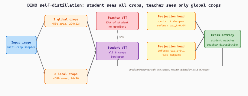
DINO operationalizes this idea through a multi-crop strategy. From each training image the data loader emits several augmented crops at two scales: two global crops covering more than 50% of the image and resized to 224x224, plus typically six local crops covering less than 50% of the image and resized to 96x96. Two copies of the same ViT process the crops: a student (parameters updated by gradient descent) and a teacher (parameters maintained as an exponential moving average of the student, with no gradients). The teacher only sees the two global crops; the student sees all crops. The target distribution is computed by passing each crop through a high-dimensional projection head (about 65,000 outputs) followed by a softmax, producing a soft pseudo-label vector. Training minimizes cross-entropy between every student crop's output and every teacher crop's output (excluding self-pairs).
The local-to-global targeting is what teaches the network semantic invariance. A 96x96 local crop of a cat's ear is forced to produce the same pseudo-label distribution as the 224x224 global crop of the whole cat, so the only way the network can satisfy both is to learn features that ignore scale and focus on shared content. Two collapse failure modes lurk: the network could output a constant distribution for every input (trivially matching itself), or it could output a peaked one-hot distribution on a single arbitrary index. DINO prevents both by centering the teacher's logits (subtract an EMA of the running mean before softmax) and sharpening them (low teacher temperature, $\tau_t \approx 0.04$). Centering prevents one dimension from dominating; sharpening prevents the trivial uniform-distribution solution.
The result is a network that has never seen a label yet produces feature maps where the [CLS] token attends cleanly to the salient object: in canonical DINO visualizations, the model trained on natural images segments cups, dogs, and birds with no segmentation supervision whatsoever. DINOv2 (covered in 22.1.6) is essentially this recipe scaled up with iBOT masked-patch losses, larger datasets, and KoLeo feature spreading regularization, but the multi-crop teacher-student core is identical.
import torch
from PIL import Image
from transformers import AutoImageProcessor, AutoModel

# Pretrained DINO ViT-B/16 (Caron et al. 2021) on ImageNet, no labels used.
processor = AutoImageProcessor.from_pretrained("facebook/dino-vitb16")
model = AutoModel.from_pretrained("facebook/dino-vitb16",
                                  output_attentions=True).eval()

image = Image.open("cat.jpg").convert("RGB")
inputs = processor(images=image, return_tensors="pt")

with torch.no_grad():
    outputs = model(**inputs)

# Last-layer attention: (batch, heads, n_tokens, n_tokens), n_tokens = 1 + 14*14
attn = outputs.attentions[-1][0]                   # (heads, 197, 197)
cls_attn = attn[:, 0, 1:]                          # CLS attends to 196 patches
cls_attn = cls_attn.reshape(-1, 14, 14).mean(dim=0)  # average over heads
print(cls_attn.shape)   # torch.Size([14, 14])
# Visualize: bright cells trace the salient object silhouette,
# even though no segmentation labels ever entered training.[CLS] token's attention to the 196 spatial patches forms a near-pixel-accurate silhouette of the dominant object, despite the model being trained without any localization labels. This is the "emerging properties" result from Caron et al. that motivated SAM, OpenSeg, and the entire post-DINO segmentation-from-features lineage.Take one cat photo, sample one global crop ($224 \times 224$, the cat's whole body) and one local crop ($96 \times 96$, just the left ear), and run a 65k-dim projection head on each. The teacher centers its global-crop logits by subtracting an EMA mean $c$ and divides by $\tau_t = 0.04$; suppose for this image the teacher's softmax peaks at $p_t \approx 0.62$ on the "cat-like cluster index" $k^* = 17{,}429$ and spreads the remaining 0.38 across the other 65k slots. The student processes the local ear crop through its own head at $\tau_s = 0.1$, producing $p_s$ with only $0.04$ probability on index 17,429 (the student has not yet learned that an ear belongs to the same cluster as a cat). The cross-entropy contribution from this index alone is $-p_t^{(k^*)} \log p_s^{(k^*)} = -0.62 \cdot \log 0.04 \approx 2.00$ nats. Summed across all 65k indices the per-pair loss is around 4.2 nats; with 8 crops per image and (8 student) x (2 teacher) - 2 self-pairs = 14 pairs the per-image loss is about 60 nats. Gradient descent on the student gradually raises $p_s^{(k^*)}$, the teacher follows via EMA ($\theta_t \leftarrow 0.996 \theta_t + 0.004 \theta_s$), and after roughly 300 ImageNet epochs the local-crop and global-crop distributions on the same image agree to within 0.02 nats per pair: the network has learned that "left ear of a cat" and "cat" should produce the same pseudo-label.
The ViT input pipeline is succinct enough to write as one equation. For an input image $x \in \mathbb{R}^{H \times W \times C}$ partitioned into $N = (H/P)(W/P)$ non-overlapping patches $x_p^i \in \mathbb{R}^{P^2 C}$, the input token sequence is
where $E \in \mathbb{R}^{P^2 C \times d}$ is the learned patch projection (implemented as a single 2D convolution with stride $P$ and kernel $P$ for efficiency), $E_{\text{pos}} \in \mathbb{R}^{(N+1) \times d}$ is the position encoding (learned in the original ViT, 2D sinusoidal or 2D-RoPE in modern variants), and $x_{\text{class}}$ is the learned $[\text{CLS}]$ token. The semicolons denote sequence concatenation. From there, $L$ standard transformer encoder blocks act on $z_0$ exactly as in BERT; the choice of pretraining objective only changes the loss applied to the final hidden states.
MAE (He et al., 2021) couples ViT with a strikingly asymmetric reconstruction objective. At training time, a random 75% subset of the $N$ patches is dropped; only the remaining 25% are fed through the encoder. A lightweight decoder (typically 8 transformer blocks, $d_{\text{dec}} = 512$, far smaller than the encoder) then receives the encoded visible tokens plus a learnable mask token at each missing position, and predicts the raw pixel values of the masked patches. The loss is mean squared error in normalized pixel space, computed only on the masked positions: $\mathcal{L}_{\mathrm{MAE}} = \tfrac{1}{|\mathcal{M}|} \sum_{i \in \mathcal{M}} \lVert x_p^i - \hat{x}_p^i \rVert_2^2$, where $\mathcal{M}$ is the set of masked patches. The 75% mask ratio is much higher than BERT's 15% because images are spatially redundant: with too small a mask the task collapses to local interpolation. The asymmetric decoder is the source of the speedup: encoder FLOPs scale with the 25% kept patches, so MAE pretrains roughly 3x faster than a same-shape contrastive encoder on equal compute.
DINOv2 (Oquab et al., 2024) uses a self-distillation scheme with an exponential-moving-average teacher. Two augmented crops of the same image are fed to a student network with parameters $\theta_s$ and a teacher with parameters $\theta_t$; the student is trained with cross-entropy to match the teacher's softened output distribution: $\mathcal{L} = -\sum_k p_t^{(k)} \log p_s^{(k)}$ where $p_t = \mathrm{softmax}((z_t - c) / \tau_t)$ uses a centered, sharpened teacher (centering $c$ is an EMA over the batch, $\tau_t \approx 0.04$). The teacher is never trained by gradient descent; its parameters are updated as $\theta_t \leftarrow m\, \theta_t + (1 - m)\, \theta_s$ with momentum $m$ ramping from 0.996 to 1.0 over training. This momentum encoder gives the student a stable, slowly-evolving target that prevents the standard self-distillation collapse where both networks predict the constant distribution. DINOv2 adds an iBOT loss (masked-patch prediction in the latent space) and a small KoLeo regularization that spreads the feature distribution over the sphere; together these produce features that segment objects without ever seeing a label. References: He et al., "Masked Autoencoders Are Scalable Vision Learners," arXiv:2111.06377 (2021); Caron et al., "Emerging Properties in Self-Supervised Vision Transformers" (DINO), arXiv:2104.14294 (2021); Oquab et al., "DINOv2," arXiv:2304.07193 (2024).
22.1.6 DINOv2 and the Shift to Self-Supervised Features
DINOv2 (Meta, 2023) deserves particular attention because it represents a different bet on what makes a good VLM vision encoder. CLIP-style encoders are explicitly text-aligned, which makes them strong on tasks that benefit from linguistic priors (object recognition, scene captioning) but weaker on tasks requiring pure visual reasoning (geometry, motion, dense correspondence). DINOv2's image-only pretraining produces features that excel on geometric and structural tasks but require more downstream alignment for language-grounded use.
The empirical 2025 consensus is that DINOv2 features beat CLIP features on segmentation, depth estimation, and dense correspondence by 8-15% mAP, while CLIP features beat DINOv2 on captioning, retrieval, and zero-shot classification by 5-10% top-1 accuracy. VLMs that need both (multimodal robotic agents, autonomous driving stacks) increasingly use both encoders in parallel.
A concrete way to picture the difference: imagine asking each encoder "where is the cup in this photo?" CLIP can tell you it sees a cup (it learned the word "cup" during training) but its bounding box drifts because the language objective never required pixel-accurate localization. DINOv2 segments the cup cleanly down to the millimeter, but if you ask it to name what it segmented, it returns "object cluster 47" because it never saw the word "cup." A robot picking up the cup needs both: CLIP says what to grab, DINOv2 says where to grab it.
The canonical DINOv2 demonstration is an attention map from the [CLS] token: for a photo of a cup on a table, the brightest attention cells form a near-pixel-accurate silhouette of the cup; for a photo of a dog on grass, the attention map outlines the dog. These maps are produced with no segmentation labels, no bounding-box supervision, and no fine-tuning. The DINOv2 paper highlights this property as the visual proof that the network has learned "what an object is" from raw pixels alone, and it is the reason DINOv2 features are now the default backbone for open-set segmentation pipelines (SAM combines a DINO-style encoder with a prompt-driven mask decoder, for instance).
22.1.6a Swin Transformer: Shifted Windows and Hierarchical Features
The plain ViT applies global self-attention over all 196 (or 577, or 1024) patch tokens. That works for image classification, where one global decision is the only thing the model has to make, but it has two structural weaknesses for dense-prediction tasks (detection, segmentation, depth). The first is cost: attention is quadratic in the token count, so doubling the input resolution quadruples the FLOPs. The second is missing multi-scale features: CNNs naturally build a feature pyramid (small features at fine resolution, large features at coarse resolution) that detectors like Faster R-CNN consume; plain ViT outputs a single resolution at every layer.
Swin Transformer (Liu et al., Microsoft Research Asia, 2021) addresses both weaknesses with two ideas: shifted local windows for cheap attention and hierarchical patch merging for CNN-pyramid-style multi-scale features. Swin became, almost overnight, the default vision backbone for dense-prediction tasks and remains so in 2026: most production detection and segmentation stacks (Mask2Former, DINO-DETR, ViTDet variants, video models) are built on a Swin or Swin-v2 backbone.
W-MSA and SW-MSA: window attention with cross-window flow
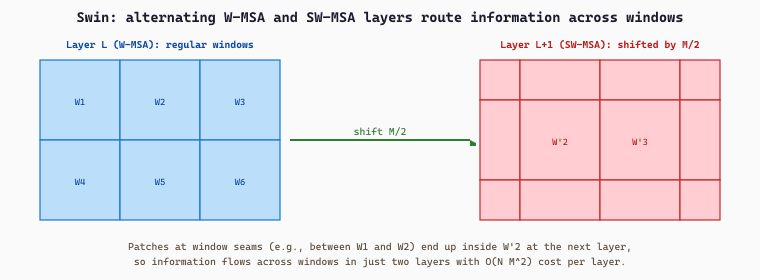
Swin replaces global self-attention with Window-MSA (W-MSA): partition the patch grid into non-overlapping windows of MxM patches (typically M=7) and run self-attention only within each window. For an HxW patch grid this drops the cost from $O((HW)^2)$ to $O(HW \cdot M^2)$, which is linear in the image area at fixed window size. The price is that windows are isolated, so information from one window never reaches another.
The cost saving is direct. For an $H \times W$ patch grid with global attention, each layer costs $\Omega(HW \cdot HW \cdot d) = \Omega((HW)^2 d)$ floating-point operations. Swin's window attention with window size $M \times M$ costs only
$$ \mathrm{FLOPs}_\mathrm{W\text{-}MSA} = \Omega\bigl(HW \cdot M^2 \cdot d\bigr), $$
which is linear in the image area at fixed $M$. The hierarchical patch-merging blocks add a constant factor: across the four stages with channel counts $C, 2C, 4C, 8C$ and grid sizes $H/4, H/8, H/16, H/32$, the total cost is dominated by stage 1 (largest grid, smallest channels) and stays approximately linear in the input pixel count.
The fix is the Shifted Window-MSA (SW-MSA) layer that alternates with W-MSA. In SW-MSA the window grid is shifted by $M/2$ patches diagonally, so patches that were on the edge of one window now sit in a new window that straddles its old neighbors. Stacking W-MSA and SW-MSA layers in pairs lets information flow across the entire image in a few steps while keeping per-layer cost linear. Conceptually, W-MSA looks within tiles and SW-MSA stitches the tiles together at the seams.
Hierarchical patch merging: a CNN pyramid built from transformer blocks
After a stack of W-MSA + SW-MSA blocks at one resolution, Swin reduces resolution and doubles the channel count through a patch merging layer. Patch merging concatenates the embeddings of every 2x2 block of neighboring patches (producing a single token with $4C$ channels), then applies a linear projection back down to $2C$ channels. The patch grid shrinks from $H \times W$ to $H/2 \times W/2$, the channel count goes from $C$ to $2C$, and the next stage's windows now cover four times the original receptive field.
Stacking four such stages produces feature maps at four resolutions (typically $H/4, H/8, H/16, H/32$) with channel counts $C, 2C, 4C, 8C$. This is exactly the shape of a CNN feature pyramid, so Swin features drop directly into Feature Pyramid Network (FPN) heads for object detection, U-Net-style decoders for segmentation, and dense prediction heads in general. Swin-T (28M params), Swin-S (50M), Swin-B (88M), and Swin-L (197M) span the same scale ladder as ResNet-50 through ResNet-200, and a Swin-L backbone replaced ResNet-50 backbones in essentially every COCO leaderboard entry within a year of release.
| Variant | Window | Hierarchical? | Attention cost | Best fit |
|---|---|---|---|---|
| Plain ViT-L/14 | global | no (single scale) | $O(N^2)$ in tokens | Classification, CLIP, VLM connectors |
| DeiT-B | global | no | $O(N^2)$ | ImageNet-1K classification, data-efficient training |
| DINOv2-L/14 | global | no | $O(N^2)$ | Self-supervised features, dense correspondence, segmentation backbones |
| Swin-L | local 7x7 + shift | yes (4 stages) | $O(N \cdot M^2)$ | Detection, instance and semantic segmentation, dense prediction |
| Swin-v2-G | local + RPE | yes | $O(N \cdot M^2)$ | 3B-param dense-prediction backbone (Microsoft 2022) |
import torch
from PIL import Image
from transformers import AutoImageProcessor, SwinModel

processor = AutoImageProcessor.from_pretrained("microsoft/swin-base-patch4-window7-224")
model = SwinModel.from_pretrained(
    "microsoft/swin-base-patch4-window7-224",
    out_features=["stage1", "stage2", "stage3", "stage4"],
).eval()

image = Image.open("street.jpg").convert("RGB")
inputs = processor(image, return_tensors="pt")
with torch.no_grad():
    outputs = model(**inputs, output_hidden_states=True)

# Four pyramid levels at H/4, H/8, H/16, H/32 with channel counts C, 2C, 4C, 8C.
for i, h in enumerate(outputs.reshaped_hidden_states):
    print(f"stage {i+1}: {tuple(h.shape)}")
# stage 1: (1, 128, 56, 56)
# stage 2: (1, 256, 28, 28)
# stage 3: (1, 512, 14, 14)
# stage 4: (1, 1024, 7, 7)Compare Swin-Base and ViT-L/14 on a 1024x1024 input, the standard COCO detection resolution. ViT-L/14 splits the image into a $1024/14 \approx 73 \times 73 = 5329$ patch grid and adds a CLS token for 5330 tokens; with $d = 1024$ each global-attention layer costs roughly $5330^2 \cdot 1024 \approx 2.9 \times 10^{10}$ FLOPs and the full 24-layer stack costs $\approx 700$ GFLOPs just for attention. Swin-B starts with a $1024/4 = 256 \times 256 = 65{,}536$ patch grid and runs window attention with $M = 7$ in four stages. Stage 1 (256x256 grid, $C = 128$) costs $65{,}536 \cdot 49 \cdot 128 \approx 4.1 \times 10^{8}$ FLOPs per layer, and across all four stages with the hierarchical 2x downsampling the total attention budget sits around 47 GFLOPs, roughly 15x cheaper than ViT-L/14 at the same resolution while producing four-level features that a Mask R-CNN head can consume directly. The Swin-B detector reaches 51.9 box mAP on COCO compared to ResNet-101's 44.0 mAP at similar compute, which is the empirical answer to "is the hierarchical structure worth the engineering complexity?".
As of 2026, the ViT zoo splits cleanly along the task axis. Plain global-attention ViTs (CLIP-ViT, SigLIP-ViT, DINOv2-ViT) dominate VLM connectors, contrastive retrieval, and self-supervised representation work, because their single-scale token sequence drops trivially into a language-model context window. Hierarchical window-attention ViTs (Swin, Swin-v2, MViT, FocalNet) dominate detection, segmentation, depth, and any task that wants an FPN-style multi-scale feature pyramid. Mixing them is fine: many production VLMs hand image inputs to SigLIP for the language-aligned token stream and to a frozen Swin backbone for an auxiliary spatial mask head, with the two feature streams concatenated at the LLM input.
22.1.7 V-NeXT and the Next Generation
The 2025-2026 generation of vision encoders pushes scale further. Two flagship examples stand out. EVA-CLIP-G (BAAI, 2024) trains a 1B-parameter ViT-G/14 on 5 billion image-text pairs and surpasses CLIP-L/14 on every zero-shot benchmark by 3 to 8 points. InternViT-6B (Shanghai AI Lab, 2024) is the largest publicly available vision encoder; InternVL 1.5 and 2.0 use it to handle 4K-resolution inputs through dynamic patch sampling.
The aggregate trend is captured by the V-NeXT family naming convention (LLaVA-NeXT, MM-NeXT, V-NeXT-T), which signals "next generation" beyond the 2023 baselines.
Two architectural innovations matter most. First, dynamic resolution and tile-based processing: rather than resizing every image to 224x224 or 336x336, modern VLMs partition large images into multiple tiles, process each through the ViT independently, and concatenate the token sequences. This preserves fine detail in high-resolution documents and dense scenes at the cost of longer sequences. Second, register tokens (Darcet et al., 2024): adding learnable tokens that do not correspond to image patches gives the model "scratch space" for cross-attention and reduces artifact tokens that otherwise appear in patch grid outputs.
In 2023, a research team training a 1B-parameter ViT noticed that ten or so patch tokens in every image converged to nearly identical, content-free embeddings, regardless of the image. These "junk tokens" turned out to be the model's emergent solution to having no proper place to store global information: it was hijacking spatially uniform patches (sky, blank backgrounds) as scratchpads. The fix (Darcet et al., 2024) was to add explicit register tokens. Adding 4-8 dedicated registers cleaned up the attention maps, improved dense prediction accuracy by 1-2%, and produced visualizations that finally made sense to humans. The lesson: when a self-attention model behaves oddly, it is often because it has no other choice given the architectural constraints.
22.1.8 Key Takeaways
- ViT turns an image into a sequence of patch embeddings (14x14 grid for 224x224 + 16x16 patches) plus a learned
[CLS]token, then runs standard transformer encoder layers. - Token count scales as (resolution/patch_size)^2; FLOPs scale quadratically in token count. This is the dominant constraint on high-resolution VLM design.
- The dominant production variant for VLMs is ViT-L/14@336 (303M params, 577 tokens), pretrained via CLIP contrastive learning.
- DINOv2 self-supervised features beat CLIP on segmentation and dense tasks; CLIP features beat DINOv2 on captioning and classification.
- DeiT showed that distilling a CNN teacher into a dedicated distillation token brings ViT training within reach of ImageNet-1K, with no JFT-300M required.
- DINO self-distillation uses two networks (student plus EMA teacher) and a multi-crop strategy (96x96 local crops matched against 224x224 global crops) to learn semantic features without labels; centering and sharpening prevent collapse.
- Swin Transformer alternates Window-MSA and Shifted-Window-MSA layers with hierarchical 2x2 patch merging, producing a CNN-style multi-scale feature pyramid that powers nearly every modern detection and segmentation backbone.
- 2025-2026 innovations include dynamic-resolution tile processing (for 4K inputs) and register tokens (for cleaner attention maps).
- EVA-CLIP-G and InternViT-6B push the frontier to 1B-6B parameter encoders, primarily serving frontier VLMs.
22.1.9 Self-Check
Show Answer
Show Answer
Show Answer
Section 22.2 dives into contrastive vision-language pretraining: how CLIP and SigLIP turn a generic ViT into a text-aligned vision encoder. This is the bedrock pretraining that powers nearly every production VLM, and the contrastive objective itself has interesting properties (zero-shot classification, retrieval, prompt engineering) that make CLIP models useful even outside of full VLM pipelines.