Efficient Multi-Tool Orchestration and Tool Economy

"The best tool call is the one you did not make, because the answer was already cached from last time."

Frontier, Cache Savvy AI Agent

27.6.1 The Cost Anatomy of a Tool Call

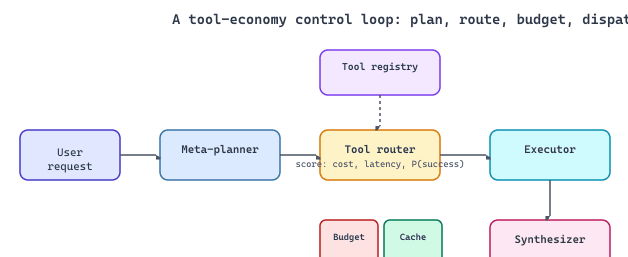
Every tool call costs you on three axes: tokens, latency, dollars. A tool-economy architecture turns these cost categories into a control loop with four moving parts:

1. Plan. A meta-planner LLM decomposes the user request into tool-shaped subgoals.
2. Route. A tool router scores candidate tools (search, compute, paid APIs, specialist sub-agents) on cost, latency, and reliability against a tool registry.
3. Budget. The router consults a budget tracker and a result cache before committing.
4. Dispatch. An executor runs the cheapest viable plan, and a synthesizer returns the final response.

Token Costs

Tokens are the cost that hides in plain sight. Tool schemas ride along in the system prompt on every call. A typical schema with three parameters runs 100 to 300 tokens. Stack 50 of them and you spend 5,000 to 15,000 tokens before the user types a word. Each round-trip adds 200 to 2,000 more tokens (reasoning + structured call + response + interpretation).

Latency & Monetary Costs

Each tool call introduces a round-trip to an external service. For local tools (file reads, calculations), this adds milliseconds. For remote APIs, this adds hundreds of milliseconds to seconds. In a multi-step agent loop, sequential calls accumulate latency that can make the system feel unresponsive. Some tools have direct per-call charges (search APIs per query, database services per read, cloud functions per invocation). At scale, these costs compound rapidly.

We can formalize the total cost of a tool call as:

where $T$ represents token counts and $P_{\text{per\_token}}$ is the price per token for the model being used.

27.6.2 Token-Efficient Tool Calling Patterns

Several engineering patterns reduce the token cost of tool use without sacrificing capability.

Dynamic Tool Loading

Rather than including all tool schemas in every request, dynamically select a subset of tools relevant to the current task. This can be done with a lightweight classifier that maps the user's query to a set of relevant tools, or by using semantic similarity between the query and tool descriptions.

from dataclasses import dataclass

@dataclass
class ToolDefinition:
    """A tool available to the agent."""
    name: str
    description: str
    schema: dict
    token_cost: int

class ToolRouter:
    """Pick top-k tools by keyword overlap; in production use embedding similarity."""
    def __init__(self, tools, max_tools=8, always_include=None):
        self.tools = {t.name: t for t in tools}
        self.max_tools, self.always_include = max_tools, set(always_include or [])
        self._kw = {t.name: set(t.description.lower().split()) for t in tools}

    def select_tools(self, query):
        qw = set(query.lower().split())
        selected = [self.tools[n] for n in self.always_include if n in self.tools]
        cands = sorted(
            ((len(qw & kw), n) for n, kw in self._kw.items()
             if n not in self.always_include and len(qw & kw) > 0),
            reverse=True,
        )
        for _, n in cands[:self.max_tools - len(selected)]:
            selected.append(self.tools[n])
        return selected

Compressed Tool Schemas & Batching

Tool descriptions are often verbose. Compressing descriptions (removing redundant words, using abbreviations, omitting obvious parameters) can reduce schema tokens by 30 to 50% without affecting the model's ability to select and use tools correctly. Frontier models are robust to compressed descriptions as long as core semantics are preserved. Tool call batching is the other big win: when an agent needs to make multiple independent tool calls, batching them into a single step (parallel tool calling) reduces the number of round-trips. Most frontier model APIs support parallel function calling.

27.6.3 Tool Caching Strategies

Many tool calls are repetitive within and across conversations. Caching tool results can eliminate redundant calls, reducing cost and latency.

Result Caching

The simplest caching strategy stores tool results keyed by tool name and arguments (SHA-256 hash). If the same tool is called with the same arguments within a configurable time window, the cached result is returned without making the actual call. This is effective for tools with deterministic or slowly-changing outputs.

Semantic Caching

For search-like tools, semantic caching stores results keyed by the semantic meaning of the query rather than the exact query string. If a user asks "What is the weather in Paris?" and then "Paris weather today?", semantic caching recognizes these as equivalent queries. Requires embedding the query and checking cosine similarity against cached queries with a configurable threshold.

import hashlib, json, time
from dataclasses import dataclass

@dataclass
class CacheEntry:
    result: str
    timestamp: float
    ttl_seconds: float
    @property
    def is_expired(self):
        return (time.time() - self.timestamp) > self.ttl_seconds

class ToolCache:
    """Exact-match cache for tool results with TTL eviction."""
    def __init__(self, default_ttl=300.0):
        self.default_ttl, self._cache = default_ttl, {}
        self._stats = {"hits": 0, "misses": 0}

    def _key(self, name, args):
        return hashlib.sha256(f"{name}:{json.dumps(args, sort_keys=True)}".encode()).hexdigest()

    def get(self, name, args):
        entry = self._cache.get(self._key(name, args))
        if entry and not entry.is_expired:
            self._stats["hits"] += 1
            return entry.result
        self._stats["misses"] += 1
        return None

    def put(self, name, args, result, ttl=None):
        self._cache[self._key(name, args)] = CacheEntry(result, time.time(), ttl or self.default_ttl)

    @property
    def hit_rate(self):
        tot = self._stats["hits"] + self._stats["misses"]
        return self._stats["hits"] / tot if tot else 0.0

27.6.4 Parallel Execution and Dependency Graphs

When an agent needs to make multiple tool calls, the optimal execution strategy depends on the dependency structure between calls. Independent calls can be executed in parallel; dependent calls must be sequential. A dependency graph for tool calls is a directed acyclic graph (DAG) where each node is a tool call and edges represent data dependencies. The optimal execution schedule is the longest path through the DAG (the critical path); all other paths can execute concurrently.

For example, consider a research agent that needs to: (1) search the web for "transformer alternatives 2025," (2) search the web for "state space models benchmarks," (3) read the top result from search 1, (4) read the top result from search 2, and (5) synthesize both readings. Calls 1 and 2 are independent (parallel); 3 and 4 depend on 1 and 2 respectively; 5 depends on both 3 and 4. The critical path is three steps, not five. Frontier model APIs increasingly support parallel function calling, where the model generates multiple tool calls in a single response.

27.6.5 Economic Models for Tool Use

Treating tool use as an economic decision means that each tool call should be evaluated against its expected benefit. For a given tool call, the expected net value is:

where $P(\text{useful})$ is the probability the tool returns information that improves the answer, $\Delta Q$ is the quality improvement, and $C_{\text{total}}$ is the total cost. A rational agent should make the call if and only if $V_{\text{net}} > 0$. When multiple tools could provide the needed information, prefer the cheapest tool that meets the quality threshold. If the agent needs current stock prices, a cached database lookup ($0.001, 10ms) is preferable to a web search ($0.01, 500ms), even if the web search might return slightly more recent data.

27.6.6 Benchmarking Tool Efficiency

Several benchmarks evaluate LLM tool use, though most focus on capability rather than efficiency. ToolBench (Qin et al., 2024) covers 16,000+ APIs but focuses on capability. API-Bank (Li et al., 2023) tests 73 APIs in a conversational setting and includes metrics for unnecessary API calls. T-Bench (Wang et al., 2024) emphasizes when to use tools versus internal knowledge and includes an efficiency score penalizing unnecessary calls. BFCL focuses on function-call accuracy without efficiency.

A comprehensive tool efficiency evaluation should include: task completion rate, tool calls per task, tokens per task, unnecessary call rate (calls that did not contribute to the final answer), parallel utilization (fraction of independent calls batched), and cache hit rate.