I finally learned to pay attention, and now I can't stop staring at every token in the sequence. My therapist calls it hypervigilance; Bahdanau calls it alignment.
Attn, Hypervigilant AI Agent
Prerequisites
This section builds directly on the encoder-decoder architecture and information bottleneck problem from Section 3.1. Understanding RNN hidden states and the seq2seq framework is essential. The intuitive introduction to attention here prepares you for the formal Q/K/V treatment in Section 3.3 and its full application in the Transformer (Section 4.1).
Why attention changed everything. In Section 3.1, we saw that the encoder-decoder architecture forces the entire source sentence through a single fixed-size bottleneck vector. Attention eliminates this bottleneck by allowing the decoder to dynamically "look back" at every encoder hidden state at every generation step. Instead of asking "what does the whole sentence mean?", the decoder can ask "which parts of the sentence are relevant right now?" This single idea, introduced in 2014 by Bahdanau et al., improved machine translation dramatically and became the foundational building block of the Transformer architecture (Chapter 4) that powers GPT, BERT, and every modern LLM.

1. The "Where to Look" Intuition
Consider a human translator converting an English sentence to French. They do not read the entire English sentence, memorize it as a single compressed thought, and then produce the French sentence from memory. Instead, they glance back at specific parts of the source sentence as they write each word of the translation. When writing the French verb, they look at the English verb. When writing the French adjective, they look at the English adjective (which might be in a different position due to word order differences between the two languages).
Attention gives neural networks this same ability. At each decoder step, the model computes a set of attention weights over all encoder positions. These weights determine how much "focus" to place on each source token. The model then takes a weighted sum of the encoder hidden states to produce a context vector that is specific to the current decoding step.
Crucially, these weights are not hardcoded. They are computed dynamically based on the decoder's current state and each encoder state. Different decoder steps attend to different parts of the source, creating a soft, differentiable alignment between source and target. Understanding how attention weights are interpreted remains an active research area, as discussed in Chapter 18: Interpretability.
Think of attention as a differentiable search engine. The decoder issues a "query" (what am I looking for?), the encoder positions are the "documents," and the attention weights are the relevance scores. Unlike a traditional search engine that returns one best match, attention returns a weighted blend of all documents, proportional to their relevance. This "soft" retrieval is what makes attention end-to-end trainable with gradient descent.
2. Bahdanau Additive Attention
The first attention mechanism for seq2seq, proposed by Bahdanau, Cho, and Bengio (2014), uses a small feedforward network (often called an alignment model) to compute the compatibility between the decoder state and each encoder state.
The Computation
Let $s_{i}$ be the decoder hidden state at step $i$, and let $h_{j}$ be the encoder hidden state at position $j$. Bahdanau attention computes:
These energy scores are normalized via softmax to produce attention weights that sum to one:
The context vector is then the weighted sum of encoder hidden states:
To make this concrete, consider a decoder attending to four source tokens with energy scores [0.2, 2.8, 0.1, 1.5]. The softmax converts these to weights, and the weighted sum produces a context vector dominated by the highest-scoring position:
# Numeric example: Bahdanau attention on 4 source tokens
import torch, torch.nn.functional as F

scores = torch.tensor([0.2, 2.8, 0.1, 1.5])
weights = F.softmax(scores, dim=0)
print(f"Scores: {scores.tolist()}")
print(f"Weights: {weights.tolist()}")
# Weights: [0.049, 0.660, 0.045, 0.246] (sum = 1.0)

# Weighted sum of 4 encoder vectors (dim=3 for brevity)
h = torch.tensor([[1.0, 0.0, 0.0], # h1
 [0.0, 1.0, 0.0], # h2
 [0.0, 0.0, 1.0], # h3
 [0.5, 0.5, 0.0]]) # h4
context = weights @ h
print(f"Context: {context.tolist()}")
# Context: [0.172, 0.783, 0.045] (dominated by h2, weight=0.66)Here is what each piece does:
- Score function $e_{ij}$: Projects both the decoder state and encoder state into a common space, adds them, applies tanh, then reduces to a scalar with $v$. This is called "additive" attention because the two projections are added together.
- Softmax normalization: Converts raw scores into a probability distribution over source positions. The weights $\alpha _{ij}$ sum to 1 and are all non-negative.
- Weighted sum: Combines encoder states according to the attention weights, producing a context vector tailored to the current decoding step.

Attention as Soft Alignment
In traditional machine translation, an alignment specifies which source word(s) correspond to each target word. Classic statistical MT systems learned hard alignments (each target word aligns to exactly one or a few source words). Attention produces a soft alignment: every target word is connected to every source word, but with varying strength.
This soft alignment has several advantages. It can handle one-to-many and many-to-one relationships naturally. It is fully differentiable, allowing end-to-end training with backpropagation. And it provides interpretability: by visualizing the attention weights as a matrix (source positions on one axis, target positions on the other), we get an alignment map that shows which source words the model "looked at" when generating each target word.
3. Luong Dot-Product Attention
Shortly after Bahdanau's work, Luong et al. (2015) proposed several alternative score functions. The most widely used is dot-product attention, which replaces the feedforward network with a simple dot product:
Luong also proposed a "general" variant that inserts a learnable matrix:
| Variant | Score Function | Parameters | Complexity |
|---|---|---|---|
| Bahdanau (additive) | vT tanh($W_{1}$s + $W_{2}$h) | O(d²) | Two projections + tanh + dot |
| Luong (dot) | sTh | 0 | Single dot product |
| Luong (general) | sTWh | O(d²) | One projection + dot |
The dot-product score is computationally cheaper and can be computed as a single matrix multiplication across all source positions simultaneously. This efficiency advantage becomes critical as we scale attention to the Transformer architecture in Section 3.3. However, note that dot-product attention requires the decoder and encoder states to have the same dimensionality, while additive attention can handle different sizes through its projection matrices.
4. Attention as a Differentiable Dictionary Lookup
The number of papers with "attention" in the title published since 2017 is itself worthy of some attention filtering. The original Bahdanau attention paper (2014) has over 30,000 citations, making it one of the most influential ideas in the history of deep learning.
There is a powerful analogy that helps unify all forms of attention: think of it as a soft dictionary lookup.
In a traditional Python dictionary, you provide a key and retrieve the exact matching value. If the key is not present, you get nothing. Attention works similarly but in a "soft" way:
- Query: What you are looking for (the decoder state $s_{i}$)
- Keys: What you compare against (the encoder states $h_{j}$)
- Values: What you retrieve (also the encoder states $h_{j}$ in Bahdanau/Luong)
Instead of exact matching, the query is compared against all keys simultaneously using a similarity function. The result is not a single value but a weighted combination of all values, where the weights reflect how well each key matches the query.
In Bahdanau and Luong attention, the keys and values are the same (both are encoder hidden states). The Transformer generalizes this by using separate linear projections to create distinct key and value representations from the same source, which is much more expressive. We will formalize this query/key/value framework in Section 3.3.
5. Implementing Attention from Scratch
Let us build both Bahdanau and Luong attention in PyTorch (Section 0.3), step by step. Code Fragment 3.2.1 below puts this into practice.
# Bahdanau (additive) attention: project decoder state and encoder outputs
# through a shared MLP, then softmax over positions to get alignment weights.
import torch
import torch.nn as nn
import torch.nn.functional as F

class BahdanauAttention(nn.Module):
 """Additive (Bahdanau) attention mechanism."""
 def __init__(self, enc_dim, dec_dim, attn_dim):
 super().__init__()
 self.W1 = nn.Linear(dec_dim, attn_dim, bias=False)
 self.W2 = nn.Linear(enc_dim, attn_dim, bias=False)
 self.v = nn.Linear(attn_dim, 1, bias=False)

 def forward(self, decoder_state, encoder_outputs):
 """
 decoder_state: (batch, dec_dim)
 encoder_outputs: (batch, src_len, enc_dim)
 Returns: context (batch, enc_dim), weights (batch, src_len)
 """
 # Expand decoder state to match encoder sequence length
 dec_proj = self.W1(decoder_state).unsqueeze(1) # (batch, 1, attn_dim)
 enc_proj = self.W2(encoder_outputs) # (batch, src_len, attn_dim)

 # Additive scoring: v^T tanh(W1*s + W2*h)
 scores = self.v(torch.tanh(dec_proj + enc_proj)) # (batch, src_len, 1)
 scores = scores.squeeze(-1) # (batch, src_len)

 # Normalize to get attention weights
 weights = F.softmax(scores, dim=-1) # (batch, src_len)

 # Weighted sum of encoder outputs
 context = torch.bmm(weights.unsqueeze(1), # (batch, 1, src_len)
 encoder_outputs) # x (batch, src_len, enc_dim)
 context = context.squeeze(1) # (batch, enc_dim)
 return context, weights

# Test it
attn = BahdanauAttention(enc_dim=128, dec_dim=128, attn_dim=64)
enc_out = torch.randn(2, 6, 128) # batch=2, 6 source tokens
dec_s = torch.randn(2, 128) # decoder state

ctx, wts = attn(dec_s, enc_out)
print(f"Context shape: {ctx.shape}")
print(f"Weights shape: {wts.shape}")
print(f"Weights sum: {wts[0].sum().item():.4f}")
print(f"Weights[0]: {wts[0].detach().numpy().round(3)}")The weights sum to 1 (as guaranteed by softmax) and the model has learned to concentrate most of its attention on positions 1 and 4 for this particular query. Now the Luong dot-product variant: Code Fragment 3.2.2 below puts this into practice.
# Luong (dot-product) attention: score = decoder_state @ encoder_outputs^T.
# Simpler and faster than Bahdanau because it skips the MLP projection.
class LuongDotAttention(nn.Module):
 """Dot-product (Luong) attention mechanism."""
 # Forward pass: define computation graph
 def forward(self, decoder_state, encoder_outputs):
 """
 decoder_state: (batch, dim)
 encoder_outputs: (batch, src_len, dim) , same dim required!
 """
 # Dot product: s^T h for each encoder position
 scores = torch.bmm(
 encoder_outputs, # (batch, src_len, dim)
 decoder_state.unsqueeze(-1) # (batch, dim, 1)
 ).squeeze(-1) # (batch, src_len)

 # Convert scores to attention weights (probabilities summing to 1)
 weights = F.softmax(scores, dim=-1)
 context = torch.bmm(weights.unsqueeze(1), encoder_outputs).squeeze(1)
 return context, weights

# Compare both mechanisms
luong_attn = LuongDotAttention()
ctx_l, wts_l = luong_attn(dec_s, enc_out)

print(f"Bahdanau weights: {wts[0].detach().numpy().round(3)}")
print(f"Luong weights: {wts_l[0].detach().numpy().round(3)}")
print(f"Both produce context of shape: {ctx_l.shape}")Notice that Luong attention produces sharper weights (more concentrated on a single position). This is because the raw dot product can produce larger magnitude scores than the bounded tanh in Bahdanau attention, leading to more peaked softmax outputs.
Understanding how attention scores are computed is only half the story. To appreciate why attention works so well as a trainable mechanism, we need to see how gradients flow through the attention computation during learning.
6. Backpropagation Through Attention
Attention is fully differentiable, which means gradients flow through it naturally during backpropagation. The key takeaway: positions that receive high attention weights also receive strong gradient signals, creating a virtuous cycle where the model learns to attend to the right places.
Advanced Deep Dive (Optional): Matrix calculus of gradient flow through attention
The Jacobian of Softmax
The attention weights are computed as $\alpha = \operatorname{softmax}(e)$. The Jacobian of softmax with respect to its input is:
where $\delta _{ij}$ is the Kronecker delta (1 if i = j, 0 otherwise). This has an important consequence: increasing score $e_{j}$ increases weight $\alpha _{j}$ but decreases all other weights (since they must sum to 1). This competitive dynamic is what makes attention selective.
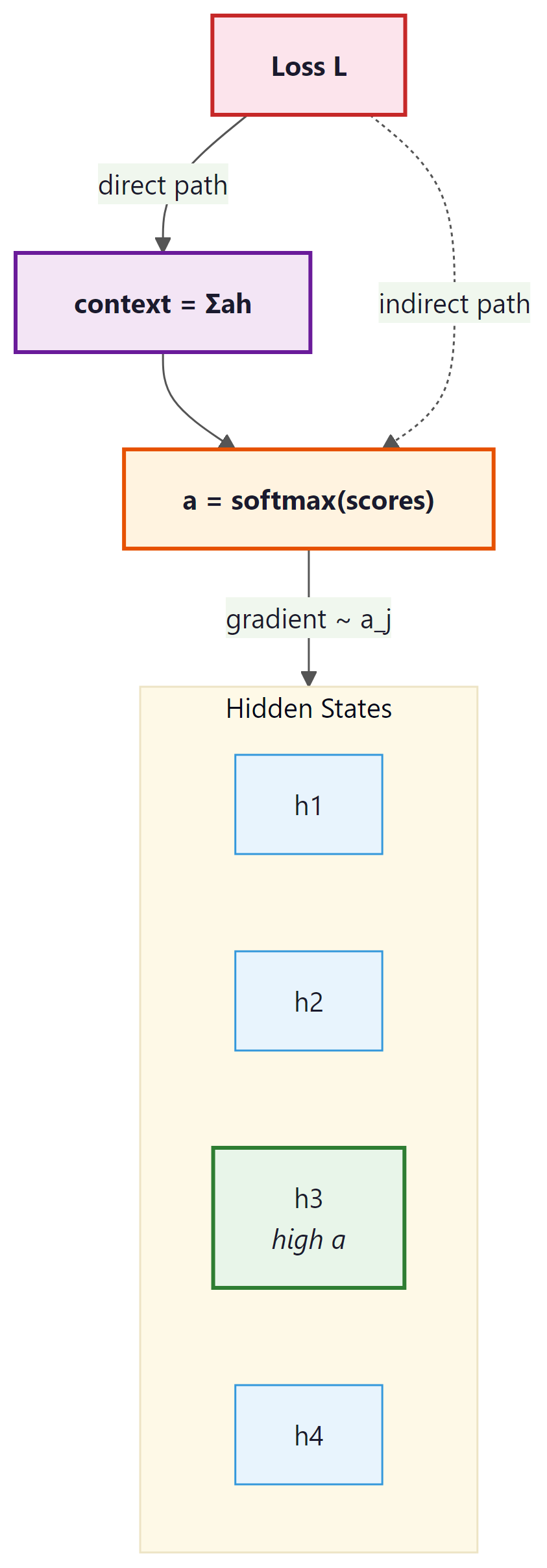
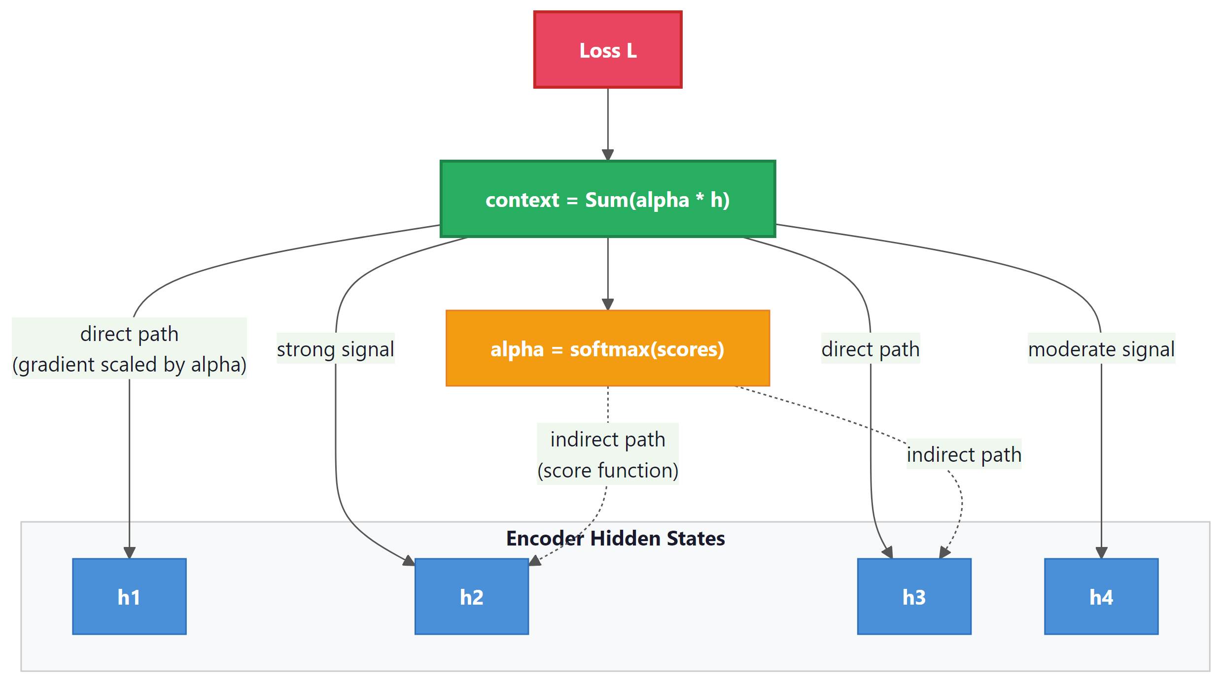
Gradient Flow Through the Context Vector
The context vector is $c = \Sigma _{j} \alpha _{j} h_{j}$. The gradient of the loss $L$ with respect to encoder state $h_{j}$ has two paths:
- Direct path: $\partial L/ \partial c \cdot \alpha _{j}$. The gradient flows directly through the weighted sum, scaled by the attention weight. Positions with high attention receive more gradient.
- Indirect path: Through the score function. Changing $h_{j}$ changes the scores, which changes the weights, which changes the context. This path allows the network to learn better scoring functions.
The direct path is analogous to a residual connection: gradient flows directly from the output back to the relevant encoder states, scaled by the attention weight. This means that positions the model attends to receive strong gradient signals, making training much more effective than in a vanilla seq2seq model where gradients must traverse the entire encoder recurrence.
Let us verify this gradient flow empirically: Code Fragment 3.2.3 below puts this into practice.
# Compare Bahdanau vs Luong attention: identical encoder outputs,
# different scoring functions. Check that gradients flow to all positions.
import torch
import torch.nn.functional as F

# Create encoder outputs with gradient tracking
enc = torch.randn(1, 5, 8, requires_grad=True) # 5 positions, dim 8
query = torch.randn(1, 8)

# Compute Luong dot-product attention
scores = torch.bmm(enc, query.unsqueeze(-1)).squeeze(-1)
weights = F.softmax(scores, dim=-1)
context = torch.bmm(weights.unsqueeze(1), enc).squeeze(1)

# Compute a scalar loss and backpropagate
loss = context.sum()
loss.backward()

print("Attention weights:", weights[0].detach().numpy().round(4))
print("Gradient norms per position:")
for j in range(5):
 grad_norm = enc.grad[0, j].norm().item()
print(f" Position {j}: weight={weights[0,j]:.4f}, grad_norm={grad_norm:.4f}")Observe the strong correlation: positions with higher attention weights receive proportionally larger gradients. Position 1, which has 78% of the attention weight, receives by far the largest gradient. This is the mechanism by which attention guides learning: the model receives the strongest training signal from the source positions it deems most relevant.
7. Integrating Attention into Seq2Seq
Now let us see how attention fits into a complete encoder-decoder model. The decoder uses the context vector (alongside its hidden state) to make predictions at each step: Code Fragment 3.2.4 below puts this into practice.
# Full attention decoder: at each step, attend over encoder outputs,
# concatenate the context vector with the embedding, and predict the next token.
import torch
import torch.nn as nn
import torch.nn.functional as F

class AttentionDecoder(nn.Module):
 """Decoder with Bahdanau attention."""
 def __init__(self, vocab_size, emb_dim, hidden_dim, enc_dim):
 super().__init__()
 self.embedding = nn.Embedding(vocab_size, emb_dim)
 self.rnn = nn.GRU(emb_dim + enc_dim, hidden_dim, batch_first=True)
 self.attention = BahdanauAttention(enc_dim, hidden_dim, attn_dim=64)
 self.fc = nn.Linear(hidden_dim + enc_dim, vocab_size)

 def forward_step(self, token, hidden, encoder_outputs):
 """One decoding step with attention."""
 # Compute attention over encoder outputs
 context, weights = self.attention(
 hidden.squeeze(0), # (batch, hidden_dim)
 encoder_outputs # (batch, src_len, enc_dim)
 )

 # Embed current token and concatenate with context
 emb = self.embedding(token) # (batch, 1, emb_dim)
 rnn_input = torch.cat([emb, context.unsqueeze(1)], dim=-1)

 # RNN step
 output, hidden = self.rnn(rnn_input, hidden) # output: (batch, 1, hidden)

 # Combine RNN output with context for prediction
 combined = torch.cat([output.squeeze(1), context], dim=-1)
 logits = self.fc(combined)
 return logits, hidden, weights

# Demo: decode 4 steps with attention
dec = AttentionDecoder(vocab_size=6000, emb_dim=64, hidden_dim=128, enc_dim=128)
enc_outputs = torch.randn(1, 8, 128) # 8 source tokens
h = torch.randn(1, 1, 128) # initial decoder hidden
tok = torch.tensor([[1]]) # <SOS>

print("Attention patterns during decoding:")
for step in range(4):
 logits, h, weights = dec.forward_step(tok, h, enc_outputs)
 tok = logits.argmax(dim=-1, keepdim=True)
 w = weights[0].detach().numpy()
 peak = w.argmax()
print(f" Step {step}: peak attention at source pos {peak} ({w[peak]:.2%})")Each decoding step focuses on a different source position, demonstrating the dynamic nature of attention. The decoder is no longer stuck with a single context vector; it constructs a fresh, step-specific context at every position.
Bahdanau attention was originally called the "alignment model" because the attention weights directly correspond to soft word alignments in translation. This connection to alignment is why the score function parameters are sometimes denoted with alignment-related variable names in the literature. Keep in mind that when the Transformer paper (Vaswani et al., 2017) uses the term "attention," it refers to the same fundamental concept but in a more general query/key/value framework that we develop in Section 3.3.
Show Answer
Show Answer
Show Answer
Show Answer
Show Answer
Neural attention mirrors the psychological concept of selective attention studied by cognitive scientists since Broadbent's filter model (1958) and Treisman's attenuation theory (1964). The human brain cannot process all sensory inputs with equal fidelity, so it allocates processing resources to the most relevant stimuli. Similarly, the softmax-weighted combination in attention is a differentiable resource allocation mechanism: the model spends its "representational budget" on the source positions most relevant to the current decision. This parallel runs deeper than analogy. Both systems face the same fundamental constraint: bounded computational resources must be distributed across an input that exceeds processing capacity. The emergence of sparse, interpretable attention patterns in trained models suggests that the mathematical structure of optimal information routing may be universal, arising independently in biological and artificial systems facing the same bottleneck.
Consider translating the French sentence "Le chat noir dort sur le tapis" into English "The black cat sleeps on the mat." Without attention, the decoder must compress all source information into a single vector. With attention, when generating "cat," the decoder assigns high weight to "chat" (position 2); when generating "black," it focuses on "noir" (position 3). This word-by-word alignment emerges naturally from training, and the resulting attention matrices serve as useful debugging tools in production translation systems. Teams at Google Translate used attention visualizations to identify systematic errors, such as the model consistently mishandling negation in long sentences.
✓ Key Takeaways
- Attention eliminates the information bottleneck by allowing the decoder to access all encoder hidden states at every step, rather than relying on a single compressed vector.
- Bahdanau (additive) attention uses a learned feedforward network to score the compatibility between decoder and encoder states. It can handle different dimensionalities but is computationally heavier.
- Luong (dot-product) attention uses a simple dot product for scoring, which is faster and can be computed as a single matrix multiplication. It requires matching dimensions.
- Attention is a soft dictionary lookup: a query (decoder state) is compared against keys (encoder states) to produce weights that determine how to combine values (also encoder states).
- Gradients flow through attention via two paths: directly through the weighted sum (scaled by α) and indirectly through the score function. This creates shortcut gradient paths that improve training.
- Attention weights are interpretable, forming soft alignment matrices that reveal which source tokens influence each target token.
Attention efficiency remains a central research concern. Linear attention methods replace softmax with kernel functions to achieve O(n) complexity. Differential Transformer (Ye et al., 2024) computes attention as the difference between two softmax attention maps, reducing noise. Native sparse attention (NSA, DeepSeek, 2025) learns sparse patterns during pretraining. The relationship between attention and in-context learning is being formalized, with results showing that attention heads implement gradient descent steps during inference.
When attention outputs look wrong, plot the attention weight matrix as a heatmap. A well-trained attention layer should show clear diagonal or structured patterns. Uniform (flat) attention usually means the layer is not learning anything useful.
What's Next?
In the next section, Section 3.3: Scaled Dot-Product & Multi-Head Attention, we formalize attention into the scaled dot-product and multi-head variants used in modern Transformers.
The paper that introduced additive attention for sequence-to-sequence models. This is the direct origin of the attention mechanism discussed in this section. Read Sections 2 and 3 for the alignment model and training details.
Introduces the dot-product (multiplicative) attention variant and compares global vs. local attention strategies. This paper provides the bridge between Bahdanau attention and the scaled dot-product used in Transformers.
The seq2seq paper that established the encoder-decoder paradigm and the information bottleneck problem that attention was designed to solve. Reading this first makes the motivation for attention much clearer.
Vaswani, A. et al. (2017). "Attention Is All You Need." NeurIPS 2017.
The Transformer paper that generalized attention into the Q/K/V framework covered in Section 3.3. Understanding Bahdanau and Luong attention from this section provides essential context for the Transformer's design decisions.
An excellent visual walkthrough of attention in seq2seq models with animated diagrams. If the mathematical formulations in this section feel abstract, this blog post provides the intuitive complement with step-by-step illustrations.