Language models are, at their core, probability machines. A transformer predicts the next token by outputting a probability distribution over the entire vocabulary. Understanding probability is therefore not optional; it is the lens through which every LLM output must be interpreted.
Probability Distributions
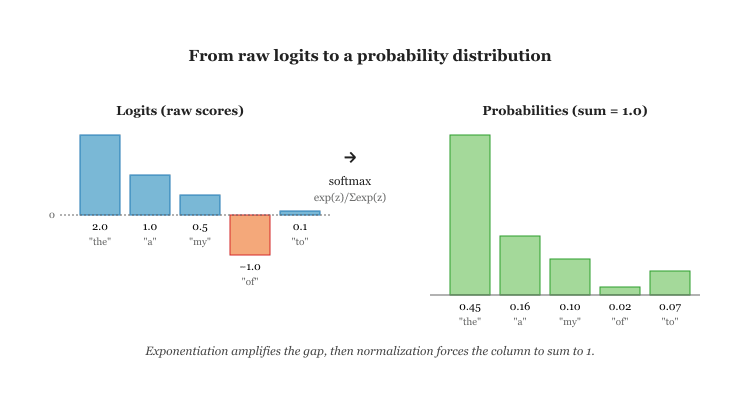
A probability distribution assigns a probability to every possible outcome such that all probabilities sum to 1. For a language model with a vocabulary of 50,000 tokens, the output at each step is a distribution over 50,000 possibilities. Code Fragment A.2.1 below puts this into practice.
# PyTorch implementation
import torch
import torch.nn.functional as F

# Raw model outputs (logits) for a vocabulary of 5 tokens
logits = torch.tensor([2.0, 1.0, 0.5, -1.0, 0.1])

# Convert to probabilities using softmax
probs = F.softmax(logits, dim=-1)
# tensor([0.4466, 0.1642, 0.0996, 0.0222, 0.0667])
# All probabilities sum to 1.0The layer normalization function is the bridge between raw model scores (logits) and probabilities:
Conditional Probability and Bayes' Theorem
Conditional probability is the probability of an event given that another event has occurred: $P(A | B) = P(A \cap B) / P(B)$. Language modeling is fundamentally about conditional probability: what is the probability of the next token given all previous tokens?
Bayes' theorem lets us reverse the direction of conditioning:
This appears in retrieval-augmented generation (RAG), where we want to find documents relevant to a query, and in classification tasks where we update beliefs about a label given observed features.
Common Distributions
| Distribution | Type | LLM Relevance |
|---|---|---|
| Categorical | Discrete | The output of softmax; used to sample the next token |
| Gaussian (Normal) | Continuous | Weight initialization, noise in diffusion models, VAE latent spaces |
| Uniform | Both | Random sampling baselines, certain initialization schemes |
| Bernoulli | Discrete | Dropout masks (each neuron kept with probability p) |
The Multivariate Gaussian
The single-variable normal distribution generalises in a straightforward way to a vector-valued random variable. The standard construction starts from a bag of independent standard normals $W_1, \dots, W_m \sim \mathcal{N}(0, 1)$, picks a mean vector $\mu \in \mathbb{R}^n$ and a matrix $A \in \mathbb{R}^{n \times m}$, and assembles the affine combination:
The covariance matrix $\Sigma = AA^T$ is automatically symmetric and positive semi-definite by construction, which is exactly the regularity needed for it to act as a covariance. When $\Sigma$ is invertible, the density of $X$ takes the canonical closed form:
This is the density behind nearly every "Gaussian" appearing later in the book: the prior over the latent code in a VAE, the noise injected at each step of a diffusion model ($x_t = \sqrt{\bar{\alpha}_t}\, x_0 + \sqrt{1 - \bar{\alpha}_t}\, \epsilon$ with $\epsilon \sim \mathcal{N}(0, I)$), the analytic prior on transformer weights used in initialisation arguments, and the kernel-form posterior of a Gaussian-process retriever.
Joint Gaussian Conditioning
The single most useful property of multivariate Gaussians is that conditioning preserves Gaussianity in closed form. Stack two jointly Gaussian vectors $X \in \mathbb{R}^n$ and $Y \in \mathbb{R}^m$ into a block-partitioned distribution:
Then the conditional distribution of $X$ given an observation $Y = y$ is again multivariate Gaussian, with a mean shift linear in the observation and a reduced covariance given by the Schur complement:
Two things deserve emphasis. First, the posterior mean is a linear regression of $X$ on $Y$ with coefficient matrix $\Sigma_{XY} \Sigma_Y^{-1}$, which is exactly the linear minimum mean-square-error (MMSE) estimator. Second, the posterior covariance is strictly smaller (in the Loewner sense) than the prior covariance whenever $\Sigma_{XY} \neq 0$, so observing a correlated variable always tightens the belief about $X$ by the Schur-complement amount, independent of the actual value of $y$.
The Gaussian conditioning identity is the workhorse behind several later constructions in this book. The closed-form forward and reverse process of diffusion models is one specific case: each step adds Gaussian noise, and the reverse-time posterior $q(x_{t-1} \mid x_t, x_0)$ is computed by exactly this formula. The Gaussian-process retrieval methods referenced in Chapter 32 compute their predictive mean and covariance the same way. The variational ELBO admits a closed-form when the variational family is Gaussian, again because of this identity. Kalman filtering, used in speech and audio pipelines, is the time-series version where $Y$ is the latest observation and $X$ the hidden state.
Expected Value and Variance
The expected value (mean) of a distribution tells you the average outcome: $E[X] = \sum x_i \cdot P(x_i)$. The variance measures spread: $Var(X) = E[(X - E[X])^2]$. Section 4.1 in transformers works by subtracting the mean and dividing by the standard deviation (the square root of variance), ensuring that activations stay in a well-behaved range throughout the network.
When generating text, the temperature parameter reshapes the probability distribution. Given logits $z$, we compute $\operatorname{softmax}(z / T)$. A temperature of 1.0 is the default distribution. Temperatures below 1.0 make the distribution sharper (more confident), while temperatures above 1.0 flatten it (more random). At $T \rightarrow 0$, the model always picks the highest-probability token (greedy decoding). At $T \rightarrow \infty$, all tokens become equally likely.