Calculus provides the machinery for training neural networks. The entire training loop, in which a model's weights are adjusted to minimize a loss function, rests on computing gradients and following them downhill.
Derivatives and Gradients
A derivative tells you how fast a function's output changes when you nudge its input. For a function $f(x)$, the derivative $f'(x)$ or $df/dx$ is the slope of the function at point $x$.
When a function has many inputs (as a loss function that depends on millions of weights), we compute partial derivatives with respect to each input. The collection of all partial derivatives is called the gradient:
The gradient points in the direction of steepest increase. To minimize the loss, we move in the opposite direction.
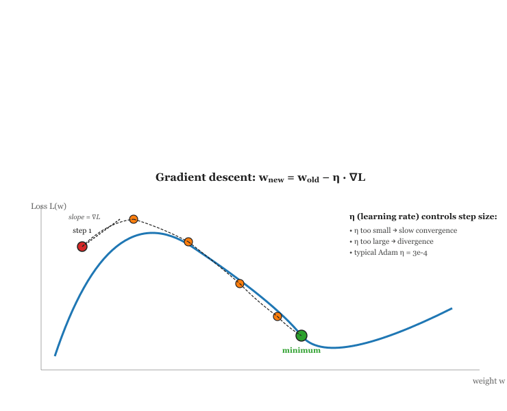
Gradient Descent
The weight update rule for cross-entropy is remarkably simple:
Here, $\eta$ (eta) is the learning rate, a small positive number that controls step size. Too large, and training diverges; too small, and convergence is painfully slow. Finding the right learning rate (and scheduling it to change over time) is one of the most important hyperparameter decisions in LLM training. Code Fragment A.3.1 below puts this into practice.
# Simplified gradient descent in PyTorch
import torch

# Suppose we have a simple loss function: L = (prediction - target)^2
w = torch.tensor([1.0], requires_grad=True)
target = torch.tensor([3.0])
learning_rate = 0.1

for step in range(10):
    prediction = w * 2.0  # simple linear model
    loss = (prediction - target) ** 2
    loss.backward()        # compute gradient

    with torch.no_grad():
        w -= learning_rate * w.grad  # update weight
w.grad.zero_() # reset gradient for next stepbackward() to obtain the gradient, updates the weight, and zeros the gradient for the next step.The Chain Rule and Backpropagation
Neural networks are compositions of many functions: the output of one layer feeds into the next. To compute how the loss depends on a weight deep in the network, we need the chain rule:
Each factor in this chain corresponds to one layer. Backpropagation is simply the efficient, automated application of the chain rule, working backwards from the loss to compute gradients for every weight in the network.
If the chain rule multiplies many factors less than 1, the gradient shrinks exponentially as it flows backward through layers (the vanishing gradient problem). If factors exceed 1, gradients explode. Techniques like layer normalization (adding the input of a layer to its output), Section 4.1, and careful initialization all exist to keep this product near 1. The transformer architecture uses residual connections around every sub-layer, which is one reason it can be trained to hundreds of layers.
The cartoon picture of gradient descent rolling into a single bowl is misleading once the parameter space has billions of dimensions. In such high-dimensional landscapes, almost every critical point with a non-trivial loss turns out to be a saddle point, not a local minimum: for a true minimum every one of the billions of curvatures has to be positive, which is statistically vanishingly rare. The empirical consequence is that vanilla SGD often slows down dramatically on saddles (the gradient is small in many directions) rather than getting trapped in spurious local minima, and the optimizers that win on transformer training (RMSprop, Adam, AdamW) all include per-parameter adaptive step sizes that explicitly help the trajectory escape these saddle plateaus. The result, first emphasised by Dauphin et al. (2014) and reinforced by every modern scaling-law paper, is that saddle escape, not local-minimum avoidance, is the real numerical challenge in deep learning.
Common Activation Functions and Their Derivatives
| Function | Formula | Derivative | Used In |
|---|---|---|---|
| ReLU | max(0, x) | 0 if x < 0, else 1 | Early transformers, CNNs |
| GELU | x · Φ(x) | Smooth approximation | BERT, GPT-2+ |
| SiLU (Swish) | x · σ(x) | Smooth, non-monotonic | LLaMA, modern LLMs |
| Sigmoid | 1 / (1 + exp(-x)) | σ(x)(1 - σ(x)) | Gating mechanisms |