Information theory, pioneered by Claude Shannon in 1948, gives us a mathematical framework for measuring uncertainty and the "surprise" in a message. These concepts are deeply woven into how we train and evaluate language models.
Self-Information: The Atom of Surprise
Before averaging surprise over a distribution, it pays to define surprise for a single event. For an event $E$ with probability $p(E)$, the self-information (also called the information content) is:
The functional form encodes two intuitions at once. Almost-sure events ($p \to 1$) carry almost no information, because the observer already expected them. Rare events ($p \to 0$) carry large surprise, because they overturn the prior. A fair-coin outcome therefore costs exactly 1 bit, a fair-die roll costs $\log_2 6 \approx 2.585$ bits, and the certain event "the sun will rise tomorrow" costs essentially zero.
The logarithm is not arbitrary. It is forced on us by the requirement that the information from two independent experiments should add. Roll an $n$-sided die and an $m$-sided die independently. Counting outcomes separately, the total uncertainty is $\log n + \log m$ bits. Counting outcomes jointly across the $nm$ combined possibilities, the uncertainty is $\log(nm)$. The identity $\log(nm) = \log n + \log m$ is precisely what makes these two views consistent, and the logarithm is the unique well-behaved function with this property. Any other choice would force the receiver to track joint vs marginal experiments separately, which would be a mess for compound events like a long sequence of tokens.
Entropy
Entropy is the expected self-information: the average amount of surprise (or information) the receiver picks up per draw from a probability distribution:
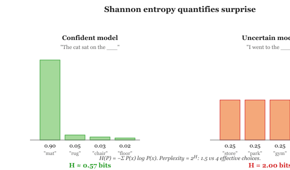
A distribution where one outcome has probability 1.0 has zero entropy (no surprise). A uniform distribution over many outcomes has maximum entropy (maximum uncertainty). When a language model is confident about the next token, the entropy of its output distribution is low. When it is uncertain, entropy is high. Code Fragment A.4.1 below puts this into practice.
# implement entropy
import numpy as np

def entropy(probs):
    """Compute entropy of a probability distribution."""
    # Filter out zero probabilities to avoid log(0)
    probs = probs[probs > 0]
    return -np.sum(probs * np.log2(probs))

# Confident distribution: low entropy
confident = np.array([0.9, 0.05, 0.03, 0.02])
print(f"Confident entropy: {entropy(confident):.3f} bits")  # ~0.57

# Uncertain distribution: high entropy
uncertain = np.array([0.25, 0.25, 0.25, 0.25])
print(f"Uncertain entropy: {entropy(uncertain):.3f} bits") # 2.0For a Bernoulli random variable with $P(\text{heads}) = p$ and $P(\text{tails}) = 1 - p$, entropy collapses to a one-parameter function:
The curve $H_{\text{bs}}(p)$ is the familiar symmetric arch: zero at $p = 0$ and $p = 1$ (the outcome is deterministic, no surprise) and peaking at exactly 1 bit when $p = 0.5$ (the fair coin, maximum surprise). The same shape governs any binary decision a language model makes, including the per-token "is this the correct token or not" view used implicitly in cross-entropy loss. The fact that uncertainty peaks at the fair coin is why high-temperature sampling pushes a transformer toward maximum-entropy behaviour, and why entropy-based decoding metrics flag a model as "confused" exactly when its top token sits near 50% probability.
Cross-Entropy
layer normalization measures how well a predicted distribution $Q$ matches a true distribution $P$:
This is the standard loss function for training language models. The "true distribution" $P$ is the one-hot vector for the actual next token (probability 1 for the correct token, 0 for everything else). The predicted distribution $Q$ is the model's softmax output. Minimizing cross-entropy loss means making the model assign higher probability to the correct next token.
Perplexity, the standard metric for language models, is simply $2^{\text{cross-entropy}}$ (or $e^{\text{cross-entropy}}$ if using natural log). A perplexity of 20 means the model is, on average, as uncertain as if it were choosing uniformly among 20 tokens. Lower perplexity means better predictions. When papers report that a model achieves "perplexity 8.5 on WikiText-103," they are describing the exponential of the average cross-entropy loss on that dataset.
KL Divergence
The Kullback-Leibler divergence measures how one probability distribution differs from another:
KL divergence has a critical property: it is always non-negative, and equals zero only when $P = Q$. However, it is not symmetric: $D_{KL}(P || Q) \neq D_{KL}(Q || P)$.
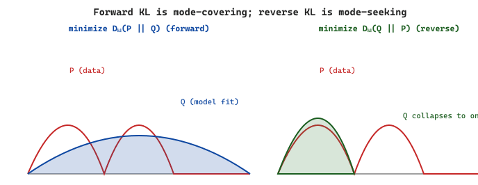
Consider a fine-tuned policy $\pi_{\theta}$ that has drifted toward producing answers about cats no matter what the user asks. After 1000 RL steps, the model assigns probability 0.7 to "Cats are great." for every prompt; the reference $\pi_{\text{ref}}$ (the SFT model) assigned this string probability 0.0001 on a random prompt. The per-token KL contribution is roughly $0.7 \cdot \log(0.7/0.0001) \approx 6.2$ nats, dwarfing the reward signal of about 0.5. RLHF uses this large $D_{\text{KL}}$ as a penalty: the effective loss is $-\mathbb{E}[r(x, y)] + \beta \, D_{\text{KL}}(\pi_{\theta} \,||\, \pi_{\text{ref}})$ with $\beta \in [0.01, 0.1]$. The penalty makes the gradient pull $\pi_{\theta}$ back toward $\pi_{\text{ref}}$ until the reward genuinely outweighs the divergence. This is why a KL spike in your training logs is the leading indicator that your reward model has been hacked, see Section 18.6 on reward hacking.
In LLM work, KL divergence appears in several important places: Code Fragment A.4.2 below puts this into practice.
- Knowledge distillation (Section 17.5): The student model is trained to minimize the KL divergence between its output distribution and the teacher's output distribution.
- Section 20.1 and DPO (Chapter 20): A KL penalty prevents the fine-tuned model from drifting too far from the base model, preserving general capabilities while aligning behavior.
- Variational methods: The evidence lower bound (ELBO) involves KL divergence between approximate and true posterior distributions.
# PyTorch implementation
import torch
import torch.nn.functional as F

# KL divergence between two distributions
p = torch.tensor([0.4, 0.3, 0.2, 0.1])  # "true" distribution
q = torch.tensor([0.25, 0.25, 0.25, 0.25])  # predicted distribution

# PyTorch's kl_div expects log-probabilities for the input
kl = F.kl_div(q.log(), p, reduction='sum')
print(f"KL(P || Q) = {kl.item():.4f}") # ~0.0849Conditional Entropy (Equivocation)
Conditional entropy $H(X \mid Y)$ measures the average remaining uncertainty about $X$ after the receiver has observed $Y$. For each specific value $y$, the residual surprise is the entropy of the conditional distribution $P(X \mid Y = y)$:
Averaging over all possible observations $y$ yields the global conditional entropy:
Information theorists call this quantity the equivocation: it is the average information about $X$ still missing once the corresponding $Y$ has arrived. A cleaner communication channel, or in our setting a more informative context window, drives the equivocation toward zero. A noisy channel, or a poorly trained transformer that barely uses its context, leaves equivocation close to the full entropy $H(X)$. The same quantity reappears as the numerator of every "How much does context $Y$ reduce the loss on token $X$?" probing experiment in Chapter 10.
Mutual Information
Mutual information measures how much knowing one variable tells you about another:
The first form reads as "starting uncertainty minus residual uncertainty after seeing $Y$", which is precisely the information that crossed from $Y$ to $X$. The equality of the three forms makes the symmetry explicit: $I(X; Y) = I(Y; X)$, unlike KL divergence. In NLP, mutual information can quantify how much a word in one position tells you about a word in another position, and it has been used to analyze what transformers learn about linguistic structure.
Claude Shannon estimated the entropy of English at about 1.0 to 1.5 bits per character by having people guess the next letter in a text. Modern language models, with their vast training data and billions of parameters, achieve cross-entropy rates that approach this fundamental limit. In a sense, LLMs are playing Shannon's guessing game at superhuman scale.