Efficient Attention, Multi-Head Reasoning & Normalization

They asked me to scale attention to a million tokens. I implemented FlashAttention. They asked for ten million. I implemented Ring Attention. They asked for a hundred million. I implemented retirement.

Attn, Memory-Bound AI Agent

Having mapped the Transformer family tree and the positional-encoding design space in Section 3.5, we now turn to the components that determine whether a Transformer can actually run at long contexts and at scale: how attention is made efficient, why multiple heads matter, and where to place LayerNorm.

3.5.3 Efficient Attention Mechanisms

Standard attention has $O(T^{2})$ time and memory complexity, where $T$ is the sequence length. For $T = 128\text{K}$ (a common context window in 2024+ models), the naive attention matrix would be $128\text{K} \times 128\text{K} = 16$ billion entries per head. This section surveys the main approaches to making attention tractable at long sequences.

3.5.3.1 Sparse Attention

Instead of attending to all positions, sparse attention restricts each token to attend to a carefully chosen subset of positions. The challenge is choosing which positions to attend to while preserving the model's ability to capture long-range dependencies.

• Local/Sliding Window Attention: Each token attends only to its neighbors within a fixed window of size $w$. Complexity becomes $O(T \times w)$. Used in Longformer and Mistral (window size 4096).
• Strided/Dilated Attention: In addition to local attention, some heads attend to every $k$-th position (dilated pattern), covering longer ranges with fewer computations. Used in BigBird and Sparse Transformer.
• Global Tokens: A small set of tokens (typically [CLS] or special sentinel tokens) attend to and are attended by all other tokens, serving as information hubs. This restores the ability to propagate information across the full sequence.

   Full quadratic              Sliding window (w=3)         Dilated sliding (w=3, stride=2)       Global tokens (cols 0, 5)
   q\k 0 1 2 3 4 5 6 7 8 9     q\k 0 1 2 3 4 5 6 7 8 9      q\k 0 1 2 3 4 5 6 7 8 9              q\k 0 1 2 3 4 5 6 7 8 9
    0  X X X X X X X X X X      0  X X . . . . . . . .       0  X . X . X . . . . .               0  X . . . . X . . . .
    1  X X X X X X X X X X      1  X X X . . . . . . .       1  X X . X . X . . . .               1  X X . . . X . . . .
    2  X X X X X X X X X X      2  X X X X . . . . . .       2  X X X . X . X . . .               2  X . X . . X . . . .
    3  X X X X X X X X X X      3  . X X X X . . . . .       3  X X X X . X . X . .               3  X . . X . X . . . .
    4  X X X X X X X X X X      4  . . X X X X . . . .       4  . X X X X . X . X .               4  X . . . X X . . . .
    5  X X X X X X X X X X      5  . . . X X X X . . .       5  . . X X X X . X . X               5  X X X X X X X X X X
    6  X X X X X X X X X X      6  . . . . X X X X . .       6  . . . X X X X . X .               6  X . . . . X X . . .
    7  X X X X X X X X X X      7  . . . . . X X X X .       7  . . . . X X X X . X               7  X . . . . X . X . .

   Time/memory: O(T^2)         Time/memory: O(T * w)        Time/memory: O(T * w)                 Time: O(T * g) with g global anchors

3.5.3.2 Linear Attention

Linear attention replaces the softmax kernel with a decomposable kernel function, allowing the attention computation to be rewritten in O(T) time:

The trick is to compute $\phi (K)^{T}V$ first (a $d \times d$ matrix, independent of T), then multiply by $\phi (Q)$. The feature map $\phi$ can be the identity (giving a simple outer-product formulation), an exponential, or a random feature approximation. Linear attention has seen renewed interest through architectures like RWKV and RetNet (discussed below).

3.5.3.3 FlashAttention

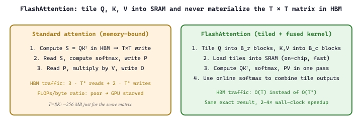
FlashAttention (Dao et al., 2022) is not an approximation; it computes exact standard attention but with dramatically better hardware utilization. The key insight is that the standard attention implementation is memory-bound: it writes the full T × T attention matrix to GPU global memory (HBM), reads it back for the softmax, writes it again, and reads it for the value multiplication. FlashAttention fuses these operations into a single kernel that keeps the attention matrix in fast on-chip SRAM, never materializing the full T × T matrix in HBM.

The result: 2 to 4x wall-clock speedup and dramatically reduced memory usage (from $O(T^{2})$ to $O(T)$ HBM). FlashAttention-2 further optimizes the kernel with better work partitioning across GPU thread blocks. FlashAttention-3 (2024) leverages Hopper GPU features (warp specialization, FP8 tensor cores) for additional gains. We cover the algorithm in detail in Section 3.6.

# Drop-in FlashAttention via PyTorch SDPA (selects the FlashAttention kernel
# automatically when the hardware and dtypes are compatible).  No math change,
# just a call into the fused kernel that the figure above describes.
import torch
import torch.nn.functional as F

torch.manual_seed(0)
B, H, T, D = 4, 16, 4096, 64                       # batch, heads, seq, head_dim
q = torch.randn(B, H, T, D, device="cuda", dtype=torch.bfloat16)
k = torch.randn_like(q)
v = torch.randn_like(q)

# Hint PyTorch to use the FlashAttention backend (PyTorch 2.2+).
with torch.backends.cuda.sdp_kernel(enable_flash=True, enable_math=False,
                                    enable_mem_efficient=False):
    out = F.scaled_dot_product_attention(q, k, v, is_causal=True)

print("output shape:", out.shape)                  # (B, H, T, D)
print("peak GPU mem MB:",
      torch.cuda.max_memory_allocated() / 1e6)      # O(T) not O(T^2)

output shape: torch.Size([4, 16, 4096, 64])
peak GPU mem MB: 268.4

3.5.3.4 Multi-Query Attention (MQA) and Grouped-Query Attention (GQA)

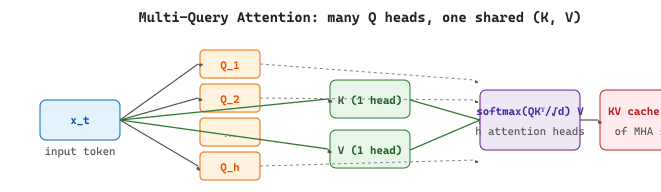
During auto-regressive inference, the keys and values from all previous positions are cached (the "KV cache"), a technique we examine in detail in Section 9.3: Memory Optimization. With standard multi-head attention and many heads, this cache becomes enormous.

• Multi-Query Attention (MQA) (Shazeer, 2019): All heads share a single set of keys and values. Only the queries differ per head. This reduces the KV cache by a factor of $h$ (the number of heads).
• Grouped-Query Attention (GQA) (Ainslie et al., 2023): A compromise where heads are divided into groups, and each group shares one set of keys and values. With $h=32$ heads and $g=8$ groups, the KV cache is reduced by 4x. Used in Llama-2, Mistral, and Gemma. For a survey of which production models use GQA, see Section 7.3.

In Hugging Face transformers, MQA is just GQA with num_key_value_heads=1, so the same config switch flips a model between the three regimes:

from transformers import AutoConfig, AutoModelForCausalLM

# Falcon-7B ships with MQA: 71 query heads share a single (K, V) pair.
cfg = AutoConfig.from_pretrained("tiiuae/falcon-7b")
print(cfg.num_attention_heads, cfg.num_kv_heads)
# 71 1   -> Multi-Query Attention

# Switch the same architecture to GQA (8 KV heads) or MHA (n_kv == n_q)
# by editing one line of the config before instantiation.
cfg.num_kv_heads = 1            # MQA  (Falcon, PaLM default)
# cfg.num_kv_heads = 8          # GQA  (Llama-2 70B, Mistral)
# cfg.num_kv_heads = cfg.num_attention_heads  # full MHA

model = AutoModelForCausalLM.from_config(cfg)

71 1

Algorithm: Generalized grouped attention (parameterized by g)
Input:  X in R^{B x T x d_model}, n_q query heads, n_kv key/value heads with
        n_q mod n_kv == 0 and group size g = n_q / n_kv
Output: Y in R^{B x T x d_model}

  // Projections: queries have full rank, KV is shared in groups
  Q := X @ W_Q                                  // (B, T, n_q,  d_k)
  K := X @ W_K                                  // (B, T, n_kv, d_k)
  V := X @ W_V                                  // (B, T, n_kv, d_k)

  // Broadcast each KV head over its group of g queries
  K_full := repeat_interleave(K, g, axis = 'head')   // (B, T, n_q, d_k)
  V_full := repeat_interleave(V, g, axis = 'head')   // (B, T, n_q, d_k)

  // Per-head scaled-dot-product attention (Algorithm 3.1.1) using K_full, V_full
  Y := concat_heads( SoftmaxAttention(Q_h, K_full_h, V_full_h) for h in 1..n_q ) @ W_O
  Return Y

Specializations:
    n_kv = n_q  (g = 1)        => MHA   (standard multi-head attention)
    n_kv = n_q / g  (1 < g)    => GQA   (LLaMA-2 70B uses n_q=64, n_kv=8, g=8)
    n_kv = 1     (g = n_q)     => MQA   (PaLM, Falcon)

KV cache per token (FP16): 2 * n_kv * d_k * 2 bytes
    MHA  (n_q=32, d_k=128): 16,384 bytes/token   (baseline)
    GQA  (n_kv=8):            4,096 bytes/token   (4x reduction)
    MQA  (n_kv=1):              512 bytes/token   (32x reduction)

from torch import nn
import torch
# Grouped-Query Attention (GQA): multiple query heads share fewer KV heads.
# Reduces KV cache size while retaining most of multi-head attention quality.
class GroupedQueryAttention(nn.Module):
    """GQA: groups of query heads share KV heads."""
    def __init__(self, d_model, n_heads, n_kv_heads):
        super().__init__()
        self.n_heads = n_heads
        self.n_kv_heads = n_kv_heads
        self.n_rep = n_heads // n_kv_heads # how many Q heads per KV head
        self.d_k = d_model // n_heads
        self.W_q = nn.Linear(d_model, n_heads * self.d_k, bias=False)
        self.W_k = nn.Linear(d_model, n_kv_heads * self.d_k, bias=False)
        self.W_v = nn.Linear(d_model, n_kv_heads * self.d_k, bias=False)
        self.W_o = nn.Linear(d_model, d_model, bias=False)
        # Forward pass: define computation graph
    def forward(self, x, mask=None):
        B, T, _ = x.shape
        q = self.W_q(x).view(B, T, self.n_heads, self.d_k).transpose(1, 2)
        k = self.W_k(x).view(B, T, self.n_kv_heads, self.d_k).transpose(1, 2)
        v = self.W_v(x).view(B, T, self.n_kv_heads, self.d_k).transpose(1, 2)
        # Repeat KV heads to match the number of query heads
        # (B, n_kv_heads, T, d_k) -> (B, n_heads, T, d_k)
        k = k.repeat_interleave(self.n_rep, dim=1)
        v = v.repeat_interleave(self.n_rep, dim=1)
        scores = (q @ k.transpose(-2, -1)) / (self.d_k ** 0.5)
        if mask is not None:
            # Mask future positions with -inf so softmax ignores them
            scores = scores.masked_fill(mask == 0, float('-inf'))
            # Convert scores to attention weights (probabilities summing to 1)
            attn = torch.softmax(scores, dim=-1)
            out = (attn @ v).transpose(1, 2).contiguous().view(B, T, -1)
            return self.W_o(out)

All the attention variants we have seen so far modify how attention scores are computed or how many heads share parameters. But they all share a common limitation: softmax attention always assigns some weight to every position, even irrelevant ones. The next approach tackles this "attention noise" problem directly.

3.5.3.5 Differential Attention (DIFF Transformer)

A more recent innovation in attention design is Differential Attention, introduced by Ye et al. (2024) in the DIFF Transformer paper. The core idea is that standard softmax attention allocates non-trivial weight to irrelevant context tokens (a phenomenon sometimes called "attention noise"). Even with a clear focus token, the long tail of softmax probabilities still assigns small but non-zero attention to unrelated positions, diluting the signal and contributing to hallucination.

Differential Attention addresses this by computing attention as the difference of two separate softmax attention maps. Each attention head is split into two sub-heads that compute independent attention distributions over the same keys, and the final attention weights are the element-wise subtraction of one from the other. Positions that receive similar attention from both sub-heads cancel out (analogous to noise cancellation), while positions that one sub-head strongly attends to but the other does not are amplified. The result is a sparser, more focused attention pattern that better distinguishes signal from noise.

import torch.nn.functional as F
import math
# Simplified Differential Attention (conceptual)
def diff_attention(Q1, K1, Q2, K2, V):
 """Two sub-attention maps; subtract to cancel noise."""
attn_1 = F.softmax(Q1 @ K1.T / math.sqrt(d_k), dim=-1)
attn_2 = F.softmax(Q2 @ K2.T / math.sqrt(d_k), dim=-1)
# Noise cancellation: positions attended equally by both cancel out
diff_weights = attn_1 - attn_2
return diff_weights @ V

Empirically, DIFF Transformers show improved performance on long-context tasks, key-value retrieval, and hallucination benchmarks, with particular gains on tasks requiring precise information extraction from noisy contexts. The approach adds minimal overhead (two sets of query/key projections per head instead of one) and is compatible with FlashAttention and GQA. Microsoft has explored integrating Differential Attention into production models, and the technique represents a promising direction for making attention more robust without fundamentally changing the Transformer architecture.

3.5.4 Multi-Head Attention: Why Multiple Heads?

We established the mechanics of multi-head attention in Section 3.1 and implemented it in Section 3.3. Now let us dig into the why: what does having multiple heads actually buy us?

The short answer is that different heads learn to attend to fundamentally different kinds of relationships, simultaneously. A single attention head produces one attention distribution over the sequence for each query position: it is forced to aggregate all of its relational reasoning into a single scalar weight per (query, key) pair. Multi-head attention runs n_heads independent attention computations in parallel, each in a lower-dimensional subspace, and then concatenates the results. This lets the model represent multiple relational modes at once.

Empirical evidence for this comes from interpretability work. Clark et al. (2019) analyzed BERT's attention patterns and found striking specialization across heads:

• Syntactic heads: some heads consistently attend from a verb to its direct object, or from a noun to its modifying adjectives, regardless of their absolute positions in the sentence.
• Coreference heads: certain heads track pronoun-antecedent relationships, attending from "she" back to the named entity it refers to, potentially dozens of tokens away.
• Local context heads: some heads attend almost exclusively to immediately adjacent tokens (a sliding-window pattern), providing a local smoothing effect.
• Global anchor heads: other heads attend heavily to special tokens like [CLS] or sentence-boundary markers, effectively routing global context signals.
• Positional heads: a subset of heads attend to fixed relative offsets (always one token back, always two tokens forward), encoding structured local order information.

Figure 3.5.8: Four types of attention head behavior observed in trained models (Clark et al., 2019). These specializations emerge from gradient descent alone; they are not explicitly programmed. Multiple heads allow the model to simultaneously represent syntactic structure, local context, global routing, and coreference, all within a single forward pass.

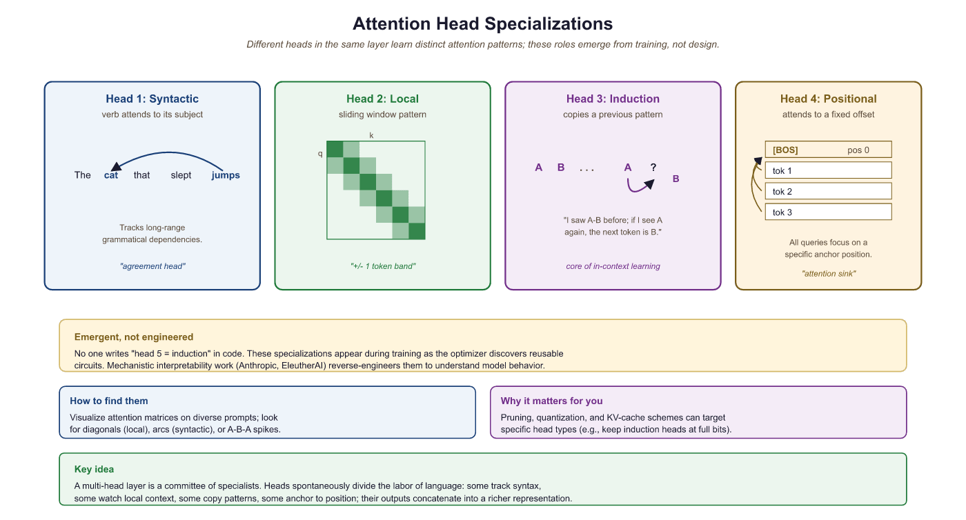
This specialization is an emergent property: no training objective explicitly requires a head to learn coreference. It arises because tracking coreference is useful for next-token prediction, and the architecture provides enough capacity (enough separate heads) for the model to allocate a head to this purpose without sacrificing others. Single-head attention cannot do this: with only one attention distribution, the model is forced to trade off between all these relational signals at every position.

For a discussion of how Grouped-Query Attention (GQA) reduces the number of key-value heads while retaining most of this multi-head representational power, see Section 9.3.

3.5.5 Pre-Norm vs. Post-Norm Layer Normalization

Layer normalization is present in every Transformer block, but where you apply it changes both training stability and model quality in ways that matter at scale. Two placement strategies have competed since 2018, and a simplified normalization variant has emerged as a third option.

3.5.5.1 Post-Norm (Original Vaswani 2017)

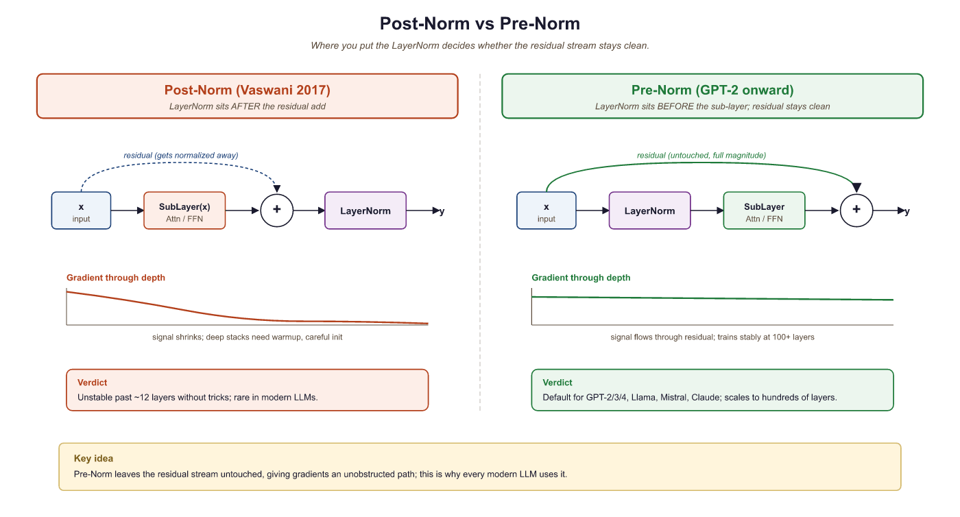
The original "Attention Is All You Need" paper placed LayerNorm after the residual add:

The intuition is clean: normalize the output of each sublayer before passing it forward. However, this placement creates a training instability problem at scale. During backpropagation, gradients flowing back to early layers must pass through the LayerNorm operations at every block. The norm statistics depend on the current activations and can produce high-variance gradients in early training before the model has settled. This forced practitioners to use very careful learning-rate warmup schedules (often thousands of steps at very low learning rate) to stabilize Post-LN training.

3.5.5.2 Pre-Norm (GPT-2 onward, all modern LLMs)

Pre-Norm applies LayerNorm before the sublayer:

The key difference: the residual path x + is not passed through LayerNorm. Gradients flowing back through the residual connection reach all earlier layers directly, without being modified by any normalization step. This produces much more stable gradient magnitudes throughout training and essentially eliminates the need for warmup warmup, or at least reduces the sensitivity to its length. Virtually every LLM trained since GPT-2 (Radford et al., 2019) uses Pre-LN. In our Section 3.3 implementation, the two lines x = x + self.attn(self.ln1(x)) and x = x + self.ffn(self.ln2(x)) are both Pre-LN.

Figure 3.5.9a: Post-Norm (left) places LayerNorm after the residual add; gradients must pass through the norm on the backward pass, causing instability at scale. Pre-Norm (right) places LayerNorm before the sublayer; the raw residual signal bypasses the norm entirely, giving stable gradients throughout training.

3.5.5.3 RMSNorm (Zhang & Sennrich, 2019)

Standard LayerNorm normalizes by subtracting the mean and dividing by the standard deviation, then scales and shifts:

RMSNorm simplifies this by removing the mean-centering step entirely and using only the root-mean-square for scaling:

The motivation: the mean-centering in standard LayerNorm re-centers activations at zero, but empirically the centering provides little or no quality benefit while adding computation. RMSNorm drops both the mean subtraction and the shift parameter $\beta$, reducing the operation to a single division and element-wise scale. Zhang and Sennrich (2019) showed that RMSNorm matches LayerNorm quality with roughly 7-12% less computation on the normalization step.

Modern LLMs have adopted RMSNorm widely. LLaMA 1 through 3, Mistral, Gemma, and Qwen all use RMSNorm in the Pre-LN position. The combination of Pre-LN placement and RMSNorm is now the de facto standard for frontier decoder-only models.

Exercises