Reducing the Footprint

"Every gigawatt-hour I do not consume is one I do not have to apologize for. Counting watts is cheaper than counting carbon."

A Frugal Optimizer, Watt-Counting AI Agent

Fun Fact: The "deploy near hydro" trick

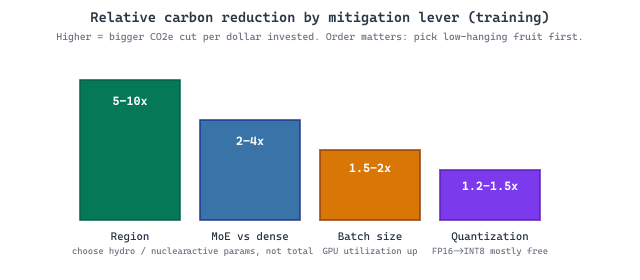
Google's GCP europe-north1 region (Hamina, Finland) draws over 95 percent of its annual energy from hydroelectric power, with the rest from wind. Routing inference there instead of us-central1 (Iowa, ~40 percent coal) can cut your per-token grid carbon by an order of magnitude with one config change and zero accuracy loss. The hard part is that data-sovereignty rules often force you back to the high-carbon region the moment your users are in the US, which is why "deploy near hydro" is half a trick and half a luxury.

55.2.1 Strategies for reducing environmental footprint

Diagnosing the problem is half the work; the other half is acting on it. Mitigation operates at three layers: the model itself (sparse architectures, distillation, quantization), the hardware substrate (efficient accelerators, optimized data centers), and the operating choices (when and where to schedule training, how to retire stale checkpoints). We treat each layer in turn, beginning with architectural choices that reduce energy at the source.

55.2.1.1 Efficient Architectures

Sparse models, particularly Mixture of Experts (MoE) architectures, activate only a fraction of their total parameters for each input token. A model like Mixtral 8x7B has 47B total parameters but activates only ~13B per token, achieving performance competitive with dense 70B models at a fraction of the inference cost. This sparsity translates directly to energy savings during both training and inference. The architecture deep dive in Chapter 8 covers MoE design in detail.

# Comparing dense vs. MoE energy efficiency
def compare_architectures(
    dense_params: float,
    moe_total_params: float,
    moe_active_params: float,
    tokens: float,
    flops_per_param_token: float = 6.0,
    hardware_tflops: float = 989.0,
    mfu: float = 0.40,
    gpu_power_w: float = 700,
    pue: float = 1.1,
    co2_g_kwh: float = 400,
    ):
    """Compare energy use of dense vs MoE models."""
    results = {}
    for name, active in [("Dense", dense_params), ("MoE", moe_active_params)]:
        total_flops = active * tokens * flops_per_param_token
        effective_tflops = hardware_tflops * mfu * 1e12
        gpu_seconds = total_flops / effective_tflops
        gpu_hours = gpu_seconds / 3600
        energy_kwh = gpu_power_w * gpu_hours / 1000 * pue
        co2_kg = energy_kwh * co2_g_kwh / 1000
        results[name] = {
            "active_params": f"{active/1e9:.0f}B",
            "energy_kwh": f"{energy_kwh:,.0f}",
            "co2_kg": f"{co2_kg:,.0f}",
            }
        dense_e = float(results["Dense"]["energy_kwh"].replace(",", ""))
        moe_e = float(results["MoE"]["energy_kwh"].replace(",", ""))
        savings = (1 - moe_e / dense_e) * 100
        results["energy_savings"] = f"{savings:.1f}%"
        return results
        result = compare_architectures(
            dense_params=70e9, moe_total_params=47e9,
            moe_active_params=13e9, tokens=2e12,
            )
        for key, value in result.items():
            print(f"{key}: {value}")

55.2.1.2 Hardware-Aware Training Decisions

Choosing the data center location based on carbon intensity is one of the highest-leverage decisions you can make. Cloud providers now expose carbon intensity data for their regions. Google Cloud's Carbon Footprint dashboard, AWS's Customer Carbon Footprint Tool, and Azure's Sustainability Calculator all provide per-region emission factors. Scheduling training runs during periods of low carbon intensity (at night in regions with significant solar capacity, or during windy periods in regions with wind farms) can further reduce emissions through a practice called carbon-aware computing.

# Carbon-aware region selection for training jobs
import dataclasses
from typing import Optional
@dataclasses.dataclass
class CloudRegion:
    name: str
    provider: str
    co2_g_kwh: float
    gpu_cost_per_hour: float
    renewable_pct: float
REGIONS = [
    CloudRegion("us-east-1", "AWS", 380, 3.06, 0.30),
    CloudRegion("us-west-2", "AWS", 120, 3.06, 0.72),
    CloudRegion("eu-north-1", "AWS", 25, 3.40, 0.95),
    CloudRegion("ca-central-1", "AWS", 30, 3.06, 0.82),
    CloudRegion("ap-south-1", "AWS", 700, 2.74, 0.18),
    CloudRegion("europe-north1", "GCP", 30, 3.22, 0.92),
    CloudRegion("us-central1", "GCP", 450, 3.22, 0.35),
    CloudRegion("swedencentral", "Azure", 20, 3.40, 0.95),
    ]
def recommend_region(
    gpu_hours: float,
    max_cost: Optional[float] = None,
    ) -> list[dict]:
    """Rank regions by carbon efficiency within budget."""
    candidates = []
    for r in REGIONS:
        cost = r.gpu_cost_per_hour * gpu_hours
        energy_kwh = 700 * gpu_hours / 1000 * 1.1
        co2_kg = energy_kwh * r.co2_g_kwh / 1000
        if max_cost and cost > max_cost:
            continue
            candidates.append({
                "region": f"{r.provider}/{r.name}",
                "co2_kg": round(co2_kg, 1),
                "cost_usd": round(cost, 0),
                "renewable": f"{r.renewable_pct:.0%}",
                })
            return sorted(candidates, key=lambda x: x["co2_kg"])
            for r in recommend_region(10_000, max_cost=50_000)[:5]:
                print(f"{r['region']:25s} CO2: {r['co2_kg']:7.1f} kg"
                    f" Cost: ${r['cost_usd']:,.0f} Renewable: {r['renewable']}")

55.2.1.3 Distillation and Quantization as Green Alternatives

Rather than training a new large model from scratch, knowledge distillation transfers capabilities from a large "teacher" model to a smaller "student" model. The student trains on the teacher's output distribution rather than raw data, requiring significantly less compute. A distilled 7B student trained to approximate a 70B teacher's behavior typically requires 10 to 100x less compute than training the 70B model originally. The efficient adaptation techniques in Chapter 17 (LoRA, QLoRA) amplify these savings further by fine-tuning only a small fraction of parameters.

Post-training quantization reduces inference energy by representing weights and activations in lower precision (INT8, INT4, or even lower). A model quantized to 4-bit precision uses roughly one-quarter the memory bandwidth and a corresponding fraction of energy per inference request. When deployed at scale across millions of daily requests, the cumulative savings are substantial.

55.2.1.4 Reusing Pretrained Models vs. Training from Scratch

The greenest training run is the one you do not perform. Using a pretrained foundation model and adapting it through fine-tuning, LoRA, or prompt engineering avoids the enormous upfront carbon cost of pretraining. A full LoRA fine-tuning run on a 7B model typically requires 1 to 10 GPU-hours, compared to 100,000+ GPU-hours for pretraining. The decision tree is simple: if an existing model can achieve your target quality with adaptation, do not train from scratch.

55.2.2 Carbon tracking tools

Carbon accounting for ML experiments requires instrumenting your training pipeline to measure energy consumption in real time. Several open-source tools make this straightforward.

55.2.2.1 CodeCarbon

CodeCarbon is the most widely adopted carbon tracking library for Python ML workflows. It monitors CPU and GPU power draw using hardware-level interfaces (RAPL for Intel CPUs, nvidia-smi for NVIDIA GPUs), combines this with the carbon intensity of your electricity grid (looked up by IP geolocation or manual configuration), and produces a CSV log of emissions per experiment.

# Tracking training emissions with CodeCarbon
from codecarbon import EmissionsTracker
from transformers import (
    AutoModelForCausalLM, AutoTokenizer,
    TrainingArguments, Trainer,
)
from datasets import load_dataset
tracker = EmissionsTracker(
    project_name="green-ai-finetune",
    output_dir="./carbon_logs",
    log_level="warning",
    measure_power_secs=30,
    tracking_mode="process",
)
tracker.start()
model_name = "meta-llama/Llama-2-7b-hf"
tokenizer = AutoTokenizer.from_pretrained(model_name)
model = AutoModelForCausalLM.from_pretrained(model_name)
dataset = load_dataset("tatsu-lab/alpaca", split="train[:1000]")
training_args = TrainingArguments(
    output_dir="./output",
    num_train_epochs=1,
    per_device_train_batch_size=4,
    gradient_accumulation_steps=4,
    fp16=True,
    logging_steps=50,
)
trainer = Trainer(model=model, args=training_args, train_dataset=dataset)
trainer.train()
emissions = tracker.stop()
print(f"\nTotal emissions: {emissions:.6f} kg CO2")
print(f"Equivalent to {emissions / 0.21:.2f} km driven")
print(f"Energy consumed: {tracker.final_emissions_data.energy_consumed:.4f} kWh")

55.2.2.2 ML CO2 Impact Calculator

For quick estimates without instrumenting your code, the ML CO2 Impact online calculator (mlco2.github.io/impact) accepts your hardware type, training duration, and cloud provider/region, then returns estimated emissions. This is useful for planning and for retrospectively estimating the footprint of experiments where you did not run a tracker.

55.2.2.3 Climatiq, Boavizta, and other carbon-accounting providers

CodeCarbon is the de-facto open-source default, but two commercial-grade alternatives are worth knowing because they cover what CodeCarbon does not:

• Climatiq (climatiq.io) is a carbon-accounting API that exposes audited emission factors for compute, networking, and embodied hardware. It accepts a JSON description of your workload (instance type, region, duration) and returns Scope 2 and Scope 3 estimates with a methodology citation. Useful when CodeCarbon's hourly granularity is not enough and you need locational-marginal or time-of-use factors.
• Boavizta (boavizta.org) is a non-profit consortium publishing open lifecycle data for computing hardware. Their boagent daemon couples power-meter telemetry with an embodied-carbon database for GPUs, motherboards, and chassis, producing per-watt Scope 3 figures that CodeCarbon's TDP heuristic cannot. This is the right tool when audit-grade reporting requires hardware-manufacturing emissions, not just operational power draw.
• WattTime and Electricity Maps provide the marginal grid intensity feeds that turn CodeCarbon's locational-average factor into a time-of-use signal. Used together, CodeCarbon plus a marginal-intensity API plus Boavizta gives a near-complete picture (operational power, real-time grid mix, embodied hardware).

Choose CodeCarbon when you need a single-import dropin; layer Climatiq or Boavizta on top when your sustainability officer needs a defensible methodology trail. All three publish their emission factors openly, which is a precondition for the EU AI Act disclosures covered in Section 55.3.

# Fetch the public ML.energy leaderboard JSON and sort by joules/token
import requests
rows = requests.get("https://ml.energy/leaderboard/api/v1/results.json").json()
best = sorted(rows, key=lambda r: r["j_per_token"])[:5] # top-5 lowest joules/token
for r in best:
    print(f"{r['model']:25s} {r['j_per_token']:6.3f} J/tok")

55.2.2.4 Experiment-Level Carbon Accounting

Integrating carbon tracking into your experiment management system (Weights and Biases, MLflow, or Neptune) allows you to compare the carbon cost of different approaches alongside their performance metrics. This enables Pareto-optimal decisions: choosing the model or hyperparameter configuration that achieves the best quality per unit of carbon emitted.

# Logging carbon metrics alongside training metrics in W&B
import wandb
from codecarbon import EmissionsTracker
def carbon_aware_training_loop(config: dict):
    """Training loop with integrated carbon tracking."""
    wandb.init(project="green-ai", config=config)
    tracker = EmissionsTracker(
        project_name=wandb.run.name, log_level="error",
        )
    tracker.start()
    for epoch in range(config["epochs"]):
        train_loss = train_one_epoch()
        val_loss = evaluate()
        current = tracker._prepare_emissions_data()
        wandb.log({
            "train/loss": train_loss,
            "val/loss": val_loss,
            "carbon/co2_kg": current.emissions,
            "carbon/energy_kwh": current.energy_consumed,
            "carbon/loss_per_co2": (
            val_loss / max(current.emissions, 1e-9)
            ),
            })
        emissions = tracker.stop()
        wandb.summary["total_co2_kg"] = emissions
        wandb.finish()

55.2.3 The rebound effect

In economics, the Jevons paradox (also called the rebound effect) observes that improvements in energy efficiency often lead to increased total energy consumption because the reduced cost per unit encourages greater usage. This pattern is playing out in the AI industry. Each generation of hardware is more energy-efficient per FLOP, yet total AI energy consumption continues to grow because the efficiency gains are reinvested into training larger models, running more experiments, and serving more inference requests.

Between 2020 and 2025, GPU energy efficiency (measured in FLOP/s per watt) improved by roughly 3x from A100 to H100/H200. During the same period, the total compute used in the largest training runs grew by approximately 10x. The net result is that total energy consumption for frontier model training increased despite hardware efficiency improvements. This pattern suggests that efficiency alone will not solve the environmental challenge; it must be combined with deliberate choices about how much compute to use.