The goal is not to build a smaller model, but to build a smaller model that remembers what the bigger one learned.
Distill, Memory-Retentive AI Agent
Knowledge distillation is the art of making small models behave like large ones. A 70B-parameter teacher model contains vast knowledge but is expensive to serve. By training a smaller student model to mimic the teacher's output distribution (not just its final answers), the student can inherit much of the teacher's capability at a fraction of the inference cost. This technique has produced some of the most remarkable results in the LLM space: Microsoft's Phi-3 models distilled from GPT-4 demonstrate that a 3.8B model can match models 10x its size. DeepSeek distilled its R1 reasoning model into compact variants that retain strong chain-of-thought abilities. The pretraining objectives from Section 6.2 explain how these teacher models acquired their knowledge in the first place.
The term "distillation" comes from chemistry: extracting the essence of a substance by heating it and collecting what evaporates. Hinton, who coined the term for neural networks, liked the metaphor because the teacher's soft probability distribution contains richer information than hard labels alone. When a teacher says "this is 70% cat, 25% tiger, 5% dog," the student learns that cats and tigers are related. Hard labels ("cat") throw away that nuance entirely.
Prerequisites
This section builds on fine-tuning from Section 16.1: When and Why to Fine-Tune and Section 6.1 covered in Section 6.1: The Landmark Models.
17.5.1 Classical Distillation Framework
Before LLM-specific distillation tricks (rationale distillation, Orca's explanation-traces, sequence-level distillation), there was Hinton's original 2015 framework: temperature-scaled softmax targets and a weighted combination of soft and hard losses. The classical setup remains the foundation, and understanding it makes every modern variant intuitive rather than mysterious.
17.5.1.1 The Teacher-Student Paradigm
Knowledge distillation mirrors a longstanding principle in pedagogy and cognitive apprenticeship theory (Collins, Brown, and Newman, 1989): experts transfer knowledge not just through explicit facts but through the structure of their reasoning. When a teacher model produces a probability distribution that assigns 0.6 to "happy" and 0.2 to "glad," the student learns not just the correct answer but the semantic neighborhood around it. This is analogous to how a master craftsperson teaches an apprentice not by listing rules but by demonstrating the full nuance of their decision-making process. In information-theoretic terms, the soft distribution contains far more bits of information than a hard label: a one-hot label carries log(V) bits (where V is vocabulary size), while a soft distribution carries the full entropy of the teacher's uncertainty. Hinton's temperature parameter directly controls how much of this "dark knowledge" is revealed, by smoothing the distribution to expose inter-class relationships that would otherwise be hidden by the winner-take-all nature of low-temperature softmax.
Knowledge distillation (Hinton et al., 2015) trains a smaller "student" model to match the output probability distribution of a larger "teacher" model, rather than training the student solely on hard ground-truth labels. Recall from Chapter 6 that a language model produces logits (raw, unnormalized scores for each token in the vocabulary) which are then converted to probabilities via the Transformer architecture function. The key insight of distillation is that the teacher's probability distribution over all possible tokens contains far richer information than a single correct answer. When the teacher assigns 0.6 probability to "happy," 0.2 to "glad," and 0.1 to "joyful," these "soft" probabilities encode semantic relationships that hard labels cannot convey. The diagram below shows this teacher-student training setup.
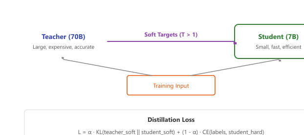
The classical Hinton distillation loss combines a temperature-softened KL term (soft targets) with a standard cross-entropy term (hard labels):
where $z_T, z_S$ are the teacher and student logits, $T$ is the temperature (typically 2 to 8), $\alpha \in [0, 1]$ weights the soft loss, and the explicit $T^2$ factor compensates for the gradient magnitude reduction caused by softening (the softmax gradient shrinks like $1/T^2$, so the factor restores its effective scale).
# Hinton-style classical knowledge distillation in PyTorch.
# The temperature smooths the teacher distribution to expose "dark knowledge"
# (relative probabilities of non-top tokens); the T^2 factor keeps the
# gradient magnitude comparable to the hard-label loss.
import torch
import torch.nn.functional as F

def kd_loss(student_logits, teacher_logits, hard_labels, T=4.0, alpha=0.5):
    # Soft-target KL between teacher and student, both softened at temperature T.
    soft_t = F.log_softmax(teacher_logits / T, dim=-1)
    soft_s = F.log_softmax(student_logits / T, dim=-1)
    loss_soft = F.kl_div(soft_s, soft_t, log_target=True, reduction="batchmean") * (T * T)
    # Standard cross-entropy on hard labels.
    loss_hard = F.cross_entropy(student_logits, hard_labels)
    return alpha * loss_soft + (1.0 - alpha) * loss_hard

# Toy step: batch of 8 examples over a 32k vocabulary.
B, V = 8, 32000
teacher_logits = torch.randn(B, V)              # frozen teacher's output
student_logits = torch.randn(B, V, requires_grad=True)
hard_labels = torch.randint(0, V, (B,))

loss = kd_loss(student_logits, teacher_logits, hard_labels, T=4.0, alpha=0.7)
loss.backward()
print("loss:", loss.item(), "| student grad norm:", student_logits.grad.norm().item())
Code Fragment 17.5.1a: Classical Hinton knowledge distillation loss in PyTorch. The T * T multiplier on the soft-target KL keeps gradients well-scaled across temperature choices; alpha trades off the teacher's "dark knowledge" against the ground-truth hard labels. White-box LLM distillation typically uses T in 2-8 and alpha in 0.5-0.9.
17.5.1.2 Temperature and Soft Targets
The temperature parameter T controls how "soft" the teacher's output distribution becomes. At T=1 (normal softmax), the teacher's distribution is peaked on the most likely token. As T increases, the distribution becomes smoother, revealing the relative probabilities of less likely tokens. This "dark knowledge" in the non-top predictions encodes the teacher's understanding of semantic similarity and uncertainty.
As illustrates, increasing the temperature gradually exposes the teacher's uncertainty across the full vocabulary, letting the student learn from the relationships between alternatives rather than just the top prediction.
Think of knowledge distillation as a master chef teaching an apprentice. The master (teacher model) does not just tell the apprentice the correct dish; they share the probability distribution over all possible dishes ('this is 70% likely a risotto, 20% a pilaf, 10% a paella'). These soft labels carry richer information than hard labels ('this is a risotto') because they reveal the master's uncertainty and the relationships between options. The apprentice (student model) learns not just the answers but the teacher's reasoning patterns, often achieving surprisingly close performance at a fraction of the size.
Knowledge distillation was first proposed by Hinton, Vinyals, and Dean in 2015. The core insight (that a teacher model's soft probability distribution carries more information than hard labels) is still the foundation of every distillation method used today.
The softmax with temperature is computed as:
where $z_{i}$ are the logits (pre-softmax values). Common temperature values range from 1.5 to 4.0. To see why temperature matters, consider logits [5.0, 2.0, 0.5] for three tokens. At T=1, softmax produces [0.92, 0.05, 0.01], a sharply peaked distribution that barely distinguishes the non-top tokens. At T=2, the distribution softens to [0.72, 0.18, 0.10], revealing that the second token is more plausible than the third. At T=4, we get [0.55, 0.26, 0.19], exposing even more of the teacher's uncertainty. Higher temperatures expose more of the teacher's knowledge but also introduce more noise. The distillation loss is scaled by T² to compensate for the gradient magnitude reduction caused by softening. Code Fragment 17.5.2 shows this approach in practice.
# Compute the KL-divergence distillation loss between teacher and student
# Soft targets from the teacher transfer more information than hard labels
import torch

import torch.nn as nn

import torch.nn.functional as F

class DistillationLoss(nn.Module):

    """Combined distillation and task loss for LLM training."""

    def __init__(self, temperature=2.0, alpha=0.5):

        super().__init__()

        self.temperature = temperature

        self.alpha = alpha # Weight for distillation vs hard label loss

        self.kl_loss = nn.KLDivLoss(reduction="batchmean")

    def forward(self, student_logits, teacher_logits, labels):

        # Soft targets: soften both distributions with temperature

        T = self.temperature

        student_soft = F.log_softmax(student_logits / T, dim=-1)

        teacher_soft = F.softmax(teacher_logits / T, dim=-1)

        # KL divergence loss (scaled by T^2)

        distill_loss = self.kl_loss(student_soft, teacher_soft) * (T ** 2)

        # Hard label cross-entropy loss

        hard_loss = F.cross_entropy(

            student_logits.view(-1, student_logits.size(-1)),

            labels.view(-1),

            ignore_index=-100,

            )

        # Combined loss

        return self.alpha * distill_loss + (1 - self.alpha) * hard_loss
{'train_loss': 1.3842, 'train_runtime': 284.7, 'train_samples_per_second': 7.02}
Distillation complete. Evaluate student against teacher.
The temperature parameter is critical. At T=1, the teacher's distribution is so peaked that it provides little more information than a hard label. At T=4, the distribution is smooth enough to reveal semantic relationships between tokens. However, too high a temperature washes out the signal entirely. Start with T=2.0 and tune based on validation performance. The T² scaling factor in the loss ensures consistent gradient magnitudes regardless of temperature.
Who: ML platform team at an e-commerce company
Situation: Product search used GPT-4 API calls to rewrite user queries into structured filters (brand, size, color, price range), processing 2 million queries per day.
Problem: GPT-4 API costs exceeded $18,000 per month, and latency averaged 1.2 seconds per query, degrading the search experience.
Dilemma: A smaller fine-tuned model could reduce cost and latency, but the team lacked labeled training data for the structured query format.
Decision: They used black-box distillation: GPT-4 generated 200,000 query-to-filter pairs from production logs, then they fine-tuned Qwen 1.5B on that synthetic dataset.
How: The student model was trained with standard cross-entropy on GPT-4 outputs (hard labels only, since logits were unavailable). Temperature-scaled soft labels were approximated by asking GPT-4 to output top-5 alternative parsings with confidence scores.
Result: The distilled 1.5B model matched GPT-4 accuracy on 94% of queries, reduced latency to 45ms (26x faster), and cut monthly costs to $400 for self-hosted inference.
Lesson: Black-box distillation from API models is a practical path to production; generating diverse synthetic training data compensates for the lack of soft probability distributions.
Why does distillation work so well? The core intuition is that a teacher model's soft probability distribution contains far more information than hard labels. When a teacher assigns probabilities [0.6, 0.2, 0.1, 0.05, 0.05] to five candidate tokens, it is implicitly encoding semantic relationships: "happy" and "glad" are closely related (both get high probability), while "table" is semantically distant (near-zero probability). A student trained on these soft targets learns these relationships in every training step, effectively receiving a compressed version of the teacher's knowledge about language structure. Hard labels ("the answer is happy") convey none of this relational information. This is why distilled models can be surprisingly capable despite being 10x smaller: they inherit the teacher's understanding of token relationships, not just its final predictions.
Distillation is fundamentally about compressing inference cost, not training cost. The distillation process itself is expensive (you must run the teacher model on your entire training set). The payoff comes at serving time, where the smaller student model delivers similar quality at a fraction of the latency and cost. This connects directly to inference optimization in Chapter 08: distillation and quantization are complementary techniques, and production deployments often apply both (distill first, then quantize the student).
17.5.2 White-Box vs. Black-Box Distillation
The distillation approach depends on what access you have to the teacher model. White-box distillation requires access to the teacher's internal logits; black-box distillation works only with the teacher's text outputs.
contrasts the two paradigms visually. The comparison table below summarizes their key differences in practice.
| Aspect | White-Box Distillation | Black-Box Distillation |
|---|---|---|
| Teacher access | Full model weights and logits | API outputs (text only) |
| Loss signal | KL (Kullback-Leibler) divergence on full distribution | Cross-entropy on generated text |
| Information richness | Very high (full probability distribution) | Lower (only top-1 output) |
| Typical teachers | Open-weight models (Llama, Mistral) | API models (GPT-4, Claude) |
| Quality ceiling | Higher (more teacher knowledge transferred) | Lower (limited to surface behavior) |
| Scalability | Limited by GPU memory for teacher | Limited by API cost and rate limits |
In practice, most LLM distillation today is black-box, simply because the most capable teachers (GPT-4, Claude) are only available through APIs. The remainder of this section examines both approaches in detail.
17.5.2.1 White-Box Distillation
When you have full access to the teacher's weights and logits, white-box distillation transfers the maximum amount of information. The following code fragment shows a complete training loop that loads both teacher and student, generates soft targets from the teacher, and trains the student on the combined loss.
# Compute the KL-divergence distillation loss between teacher and student
# Soft targets from the teacher transfer more information than hard labels
import torch

from transformers import AutoModelForCausalLM, AutoTokenizer

from torch.utils.data import DataLoader

def white_box_distillation(

    teacher_model_id: str,

    student_model_id: str,

    train_dataset,

    temperature: float = 2.0,

    alpha: float = 0.5,

    epochs: int = 3,

    lr: float = 2e-5,

    ):

    """Train student to match teacher logit distribution."""

    # Load teacher (frozen, in eval mode)

    teacher = AutoModelForCausalLM.from_pretrained(

        teacher_model_id, torch_dtype=torch.bfloat16, device_map="auto"

        )

    teacher.eval()

    for param in teacher.parameters():

        param.requires_grad = False

        # Load student (trainable)

        student = AutoModelForCausalLM.from_pretrained(

            student_model_id, torch_dtype=torch.bfloat16, device_map="auto"

            )

        loss_fn = DistillationLoss(temperature=temperature, alpha=alpha)

        optimizer = torch.optim.AdamW(student.parameters(), lr=lr)

        dataloader = DataLoader(train_dataset, batch_size=4, shuffle=True)

        for epoch in range(epochs):

            student.train()

            total_loss = 0

            for batch in dataloader:

                input_ids = batch["input_ids"].to(student.device)

                labels = batch["labels"].to(student.device)

                # Get teacher logits (no gradient)

                with torch.no_grad():

                    teacher_out = teacher(input_ids=input_ids)

                    teacher_logits = teacher_out.logits

                    # Get student logits

                    student_out = student(input_ids=input_ids)

                    student_logits = student_out.logits

                    # Compute combined loss

                    loss = loss_fn(student_logits, teacher_logits, labels)

                    loss.backward()

                    optimizer.step()

                    optimizer.zero_grad()

                    total_loss += loss.item()

                    print(f"Epoch {epoch+1}: avg_loss = {total_loss/len(dataloader):.4f}")

return student17.5.2.2 Black-Box Distillation
When the teacher is an API model (GPT-4, Claude, Gemini), you cannot access logits. Instead, you generate a large dataset of high-quality (input, output) pairs from the teacher, then fine-tune the student on these pairs using standard supervised training. The quality of the distilled student depends heavily on the diversity and quality of the generated training data. Code Fragment 17.5.5 shows this in practice.
# Generate teacher labels asynchronously for large-scale distillation
# Async batching maximizes throughput when labeling with an API-based teacher
import asyncio

from openai import AsyncOpenAI

import json

client = AsyncOpenAI()

async def generate_distillation_data(

    prompts: list[str],

    teacher_model: str = "gpt-4o",

    system_prompt: str = "You are a helpful assistant.",

    max_concurrent: int = 10,

    ) -> list[dict]:

    """Generate training data from API teacher for black-box distillation."""

    semaphore = asyncio.Semaphore(max_concurrent)

    results = []

async def call_teacher(prompt):

    async with semaphore:

        response = await client.chat.completions.create(

            model=teacher_model,

            messages=[

            {"role": "system", "content": system_prompt},

            {"role": "user", "content": prompt},

            ],

            temperature=0.7,

            max_tokens=2048,

            )

        return {

            "instruction": prompt,

            "response": response.choices[0].message.content,

            "teacher": teacher_model,

            }

        tasks = [call_teacher(p) for p in prompts]

        results = await asyncio.gather(*tasks, return_exceptions=True)

        # Filter out errors

        valid = [r for r in results if isinstance(r, dict)]

        print(f"Generated {len(valid)}/{len(prompts)} training examples")

        return valid

        # Generate dataset

        # training_data = asyncio.run(generate_distillation_data(prompts))

        # Then fine-tune student model on this data using standard SFT
Black-box distillation from proprietary API models raises important licensing considerations. Most API providers (OpenAI, Anthropic, Google) have terms of service that restrict using their outputs to train competing models. Always review the provider's usage policy before conducting distillation. Open-weight models (Llama, Mistral, Qwen) generally allow distillation, but check their specific licenses. The Llama-3 license, for example, allows derivative works but has specific restrictions for very large deployments.
17.5.3 Case Studies in LLM Distillation
Theory and recipes only carry conviction once you see them succeed in shipped models. The next three case studies (Orca, Phi, and DistilBERT) each pushed a different dial: Orca proved reasoning traces transfer, Phi proved curated synthetic data can beat raw scale, and DistilBERT proved encoder distillation can preserve 97% of the original's capability at 40% of its parameters.
17.5.3.1 Orca: Learning from Complex Explanations
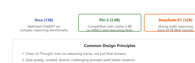
Microsoft's Orca (2023) demonstrated that small models can dramatically improve by learning not just the teacher's answers but its reasoning process. Orca trained a 13B student on millions of examples from GPT-4 that included detailed chain-of-thought explanations, step-by-step reasoning, and self-correction. The key innovations were: using system prompts to elicit rich explanations from the teacher, curating diverse and challenging prompts, and training the student on the full reasoning trace rather than just the final answer.
17.5.3.2 Phi Series: Textbook-Quality Data
Microsoft's Phi models (Phi-1, Phi-1.5, Phi-2, Phi-3) showed that data quality matters more than model size. Rather than distilling on conversational data, the Phi team used GPT-4 to generate "textbook-quality" synthetic training data: carefully structured explanations, worked examples, and exercises across diverse topics. Phi-3 (3.8B parameters) achieves performance competitive with much larger models on reasoning benchmarks, demonstrating that a small model trained on exceptional data can outperform a larger model trained on mediocre data.
17.5.3.3 Distilled DeepSeek-R1
DeepSeek distilled their large R1 reasoning model (671B MoE) into a family of smaller dense models (1.5B, 7B, 8B, 14B, 32B, 70B). The distillation process used 800K samples of the R1 teacher's chain-of-thought reasoning traces. The distilled models retain strong mathematical and coding reasoning abilities, with the 32B distilled variant outperforming many larger models on math benchmarks. This demonstrates that reasoning capabilities, which were previously thought to require enormous scale, can be effectively compressed through distillation. The table below summarizes the key principles shared by successful distillation projects.
The single most impactful lesson from distillation research is: distill the reasoning process, not just the answer. When a teacher model generates chain-of-thought explanations, step-by-step solutions, and self-corrections, the student learns much more effectively than from answer-only training data. This is why models like Orca and distilled DeepSeek-R1 dramatically outperform naive distillation approaches that only collect the teacher's final outputs.
17.5.3.4 DistilBERT: The Original Three-Term Distillation Loss
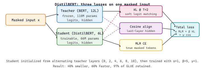
DistilBERT (Sanh et al., 2019) is the canonical encoder distillation case study and remains the textbook example of multi-term distillation. The student halves the depth of BERT-base (6 transformer blocks vs 12) and removes the next-sentence-prediction head, giving 66M parameters against BERT's 110M (a 40 percent shrink) while preserving roughly 97 percent of the original's GLUE score. The student is initialized by copying alternating layers of the teacher (layers 0, 2, 4, 6, 8, 10), then trained on the same masked-language-modeling corpus the teacher saw, with a loss that is the weighted sum of three terms:
- $\mathcal{L}_{\text{MLM}}$ is the standard masked-language-modeling cross-entropy against the true masked tokens (the same loss used to pretrain BERT).
- $\mathcal{L}_{\text{KL}}$ is the temperature-scaled KL divergence between the student's and the teacher's softmax distributions at each masked position, using the soft-target trick from Section 17.5.1.2 with $T = 2$.
- $\mathcal{L}_{\text{cos}}$ is a cosine embedding loss that pushes the student's last-layer hidden states to point in the same direction as the teacher's, transferring representation geometry alongside token-level probabilities.
Sanh et al. report a weighting of roughly $\alpha = 1.0$, $\beta = 5.0$, $\gamma = 1.0$ in the original paper, with the KL term dominating because it carries the richest signal. The cosine term is the under-appreciated piece: it constrains the student to inhabit the same representation manifold as the teacher, which is what lets shallow students transfer cleanly to downstream tasks via the standard [CLS]-pooling fine-tune recipe. The DistilBERT recipe generalizes beyond BERT (DistilGPT-2, DistilRoBERTa, TinyBERT all use the same three-term template) and is the historical bridge from Hinton's 2015 soft-target idea to the multi-term losses used by every modern distillation pipeline.
The code fragment below sketches the three-term loss as it actually appears in a DistilBERT-style training step.
# DistilBERT-style three-term loss for masked-language-modeling distillation.
import torch
import torch.nn.functional as F

def distilbert_loss(student_logits, teacher_logits, student_hidden, teacher_hidden,
                    labels, mask, T=2.0, alpha=1.0, beta=5.0, gamma=1.0):
    # Term 1: standard MLM cross-entropy on the true masked tokens.
    mlm = F.cross_entropy(student_logits.view(-1, student_logits.size(-1)),
                          labels.view(-1), ignore_index=-100)
    # Term 2: temperature-scaled KL between student and teacher token distributions.
    s_logp = F.log_softmax(student_logits / T, dim=-1)
    t_p    = F.softmax(teacher_logits / T, dim=-1)
    kl     = F.kl_div(s_logp, t_p, reduction="batchmean") * (T * T)
    # Term 3: cosine alignment of last-layer hidden states (transfers geometry).
    s_h = student_hidden[mask.bool()]
    t_h = teacher_hidden[mask.bool()]
    cos = (1.0 - F.cosine_similarity(s_h, t_h, dim=-1)).mean()
    return alpha * mlm + beta * kl + gamma * cos
The flow of the three supervisory signals through the teacher and student is summarised in Figure 17.5.3a: a single masked input is run through both networks, and the student receives three gradients in parallel.
In practice, the distilled student is treated as any other Hugging Face encoder: load the pretrained checkpoint, add a task head, hand both to Trainer. Code Fragment 17.5.2b shows the canonical fine-tune of DistilBERT on a sequence-classification task.
# Fine-tuning DistilBERT for sequence classification, the deployable shortcut.
from transformers import (DistilBertForSequenceClassification, DistilBertTokenizerFast,
                          Trainer, TrainingArguments)
from datasets import load_dataset

tok = DistilBertTokenizerFast.from_pretrained("distilbert-base-uncased")
model = DistilBertForSequenceClassification.from_pretrained("distilbert-base-uncased", num_labels=2)
ds = load_dataset("imdb").map(lambda b: tok(b["text"], truncation=True, padding="max_length"), batched=True)
args = TrainingArguments("./distilbert-imdb", per_device_train_batch_size=16,
                         num_train_epochs=1, learning_rate=5e-5, fp16=True)
Trainer(model=model, args=args, train_dataset=ds["train"].select(range(2000))).train()
Code Fragment 17.5.2c: Drop-in fine-tune of distilbert-base-uncased. The student inherits BERT's tokenizer and API, so existing pipelines swap one from_pretrained string and gain roughly 2x throughput.
Concretely, BERT-base has 12 transformer blocks, hidden size 768, 12 attention heads, and 110M parameters. DistilBERT keeps the same hidden size and head count but halves the depth to 6 blocks and drops the next-sentence-prediction head, yielding 66M parameters (a 40% reduction). On the GLUE benchmark, BERT-base scores 79.5 (average across 9 tasks) and DistilBERT scores 77.0, a relative retention of $77.0 / 79.5 \approx 97\%$. Inference latency on a CPU drops from roughly $410$ ms to $170$ ms per query (about 2.4x faster), and the model now fits in 250 MB of FP16 storage instead of 440 MB. The price paid is concentrated in tasks that require deep multi-step reasoning (the depth halving costs about 4 points on MNLI but less than 1 point on SST-2 sentiment classification); the cosine term in $\mathcal{L}_{\text{DistilBERT}}$ is what keeps the [CLS]-pooled vectors close enough to BERT's that downstream fine-tunes still converge in the standard recipe with no architectural change.
17.5.4 Small-but-Capable Models
Distillation has enabled a new class of small models that achieve remarkable performance relative to their size. These models demonstrate that the right combination of architecture, training data, and distillation can produce efficient models for deployment on edge devices, mobile platforms, or high-throughput serving scenarios.
| Model Family | Sizes | Key Technique | Notable Capability |
|---|---|---|---|
| Phi (Microsoft) | 1.3B, 2.7B, 3.8B, 14B | Textbook-quality synthetic data | Strong reasoning for size |
| Gemma (Google) | 2B, 7B, 9B, 27B | Distilled from Gemini | Multilingual, coding |
| SmolLM (HF) | 135M, 360M, 1.7B | Curated web + synthetic data | Ultra-small deployment |
| Qwen2.5 (Alibaba) | 0.5B, 1.5B, 3B, 7B+ | Multi-stage distillation | Math, code, multilingual |
| Llama-3.2 (Meta) | 1B, 3B | Pruning + distillation | On-device, mobile |
Beyond Distillation: Training Efficient Small Models Directly
Not all small, capable models are created through distillation. Several complementary approaches produce efficient models by rethinking how small models are trained from scratch or derived from larger ones.
- Sheared LLaMA (Xia et al., 2023) uses structured pruning to derive smaller models from larger pretrained ones. Rather than training a 1.3B model from scratch, the approach starts with Llama-2 7B and removes entire attention heads, layers, and hidden dimensions guided by importance scores. The pruned model is then briefly retrained on a small data budget, producing a 1.3B model that outperforms one trained from scratch with equivalent compute.
- MiniCPM (Hu et al., 2024) demonstrates that 2B-parameter models can achieve performance comparable to 7B models through careful training recipe optimization: WSD learning rate scheduling, high-quality data mixtures, and extended training well beyond the Chinchilla-optimal token count.
- The Phi family (Microsoft) makes the strongest case that data quality can substitute for model size. Phi-1 (1.3B) matched GPT-3.5 on code generation by training on "textbook-quality" synthetic data. Phi-2 (2.7B) and Phi-3 (3.8B) extended this approach, consistently outperforming models 5x their size on reasoning benchmarks.
The common thread is the Chinchilla lesson applied at small scale (see Section 6.3): an undertrained 7B model is often worse than a well-trained 2B model. For deployment on edge devices and cost-sensitive applications, these approaches complement the distillation and quantization techniques from Section 9.1.
The aha: a teacher's 70B weights spread its capacity across thousands of tasks (poetry, code, trivia, multiple languages, role-play). When you distill only math reasoning traces into a 7B student, every parameter is now dedicated to math. The student inherits the teacher's reasoning style (chain-of-thought, self-correction) while shedding everything else. So on a narrow benchmark, the 7B specialist beats the 70B generalist not because it knows more, but because it stopped storing what it does not need. Distillation acts as forced specialization: the teacher's "essence" for one domain, compressed into a model whose capacity is no longer diluted.
17.5.5 Practical Distillation Pipeline
Here is a complete pipeline that combines data generation from an API teacher with student training, demonstrating the end-to-end black-box distillation workflow. Code Fragment 17.5.3c shows this approach in practice.
# Load and prepare the distillation dataset with teacher-generated labels
# Each example pairs an input with the teacher model's soft predictions
from datasets import Dataset

from transformers import AutoModelForCausalLM, AutoTokenizer

from trl import SFTTrainer, SFTConfig

from peft import LoraConfig

import json

# Step 1: Prepare distillation dataset

# (Assume we have generated data from teacher API)

distillation_data = [

 {

 "messages": [

 {"role": "user", "content": "Explain gradient descent."},

 {"role": "assistant", "content": "Gradient descent is an optimization..."},

 ]

 },

 # ... thousands more examples

]

dataset = Dataset.from_list(distillation_data)

# Step 2: Configure student with LoRA (parameter-efficient)

student_id = "meta-llama/Llama-3.2-3B-Instruct"

tokenizer = AutoTokenizer.from_pretrained(student_id)

lora_config = LoraConfig(

 r=32, # Higher rank for distillation

 lora_alpha=64,

 target_modules="all-linear",

 task_type="CAUSAL_LM",

)

# Step 3: Train student on teacher-generated data

sft_config = SFTConfig(

 output_dir="./distilled-student",

 num_train_epochs=3,

 per_device_train_batch_size=4,

 gradient_accumulation_steps=4,

 learning_rate=2e-4,

 bf16=True,

 max_seq_length=4096,

 logging_steps=10,

 save_strategy="epoch",

)

trainer = SFTTrainer(

 model=student_id,

 args=sft_config,

 train_dataset=dataset,

 peft_config=lora_config,

)

trainer.train()

print("Distillation complete. Evaluate student against teacher.")For distillation, use a higher LoRA rank (32-64) than you would for standard fine-tuning. The student needs more capacity to absorb the teacher's knowledge. Also consider training for more epochs (3-5) with a larger and more diverse dataset. Distillation benefits from data scale more than standard fine-tuning because each example conveys information about the teacher's behavior across many dimensions.
Distill a 7B teacher into a 1.5B student on 5K instruction examples using temperatures T in {1, 2, 4, 8} on the soft-target term. Plot teacher-student KL divergence at the end of epoch 1 against task accuracy on a 500-example holdout. Identify the T that maximizes student accuracy.
Answer Sketch
Typical pattern: T=1 underuses soft targets (KL stays low but student behaves like an SFT model on hard labels), T=8 over-smooths (student picks up teacher's noise), and T=2 to 4 is the sweet spot. The hinton paper recommends T in this range, and current LLM distillation work (DistilBERT, Orca) converges on the same band. Don't forget the T^2 scaling factor on the KL term when comparing across temperatures.
You can distill from GPT-4 (black-box, $30 per million output tokens, only top logprobs visible) or from a local Llama-3-70B (white-box, full logits, $0 cash but 8 hours of GPU time on 4xA100). For a 200K-example student dataset, compute the dollar cost of each path and identify one task type where black-box still wins despite the cost.
Answer Sketch
Black-box: 200K examples x 300 tokens output ≈ 60M tokens x $30/M ≈ $1,800, plus you only see top-5 logprobs. White-box: 4xA100 at $6/hr x 8 hrs ≈ $192, full logits. White-box wins on cost roughly 9x. Black-box still wins for capabilities that the 70B teacher lacks (frontier reasoning, code generation in niche languages, multilingual fluency) because the student inherits the teacher's ceiling.
What's Next?
In the next part of this section, Section 17.6: Distillation: Licensing, Speculative & Reasoning, we step beyond the basic pipeline to three production-relevant topics: the provider licensing terms that determine whether you may distill at all, speculative distillation as an inference-time accelerator, and chain-of-thought distillation that transfers reasoning capability into smaller students.