"Every prediction has a story. Attribution methods are how we make the model tell it."
Probe, Story Extracting AI Agent
No single explanation method tells the whole truth about a Transformer architecture's predictions. Raw attention weights, gradient-based attribution, attention rollout, and perturbation methods each capture different aspects of how information flows through the network. Understanding the strengths, limitations, and failure modes of each method is essential for choosing the right tool and interpreting results correctly. This section provides a systematic comparison framework for transformer explanation methods, helping practitioners select approaches that match their specific needs. The individual methods from Section 10.1 and Section 10.3 are the techniques being compared here.
Prerequisites
Before starting, make sure you are familiar with interpretability fundamentals as covered in Section 10.1: Attention Analysis and Probing.
10.4.1 The Explanation Problem
Sparse autoencoders (SAEs) decompose model activations into a dictionary of monosemantic features. The standard L1-penalised SAE recovers many interpretable features but suffers from "feature shrinkage" (the L1 penalty pulls activations toward zero, biasing reconstruction). 2024 TopK SAEs (Gao et al., Templeton et al.) replace the L1 penalty with a hard top-K selection per token, removing shrinkage at the cost of a fixed sparsity level rather than a learned one. The open question is the bias-variance tradeoff: TopK reduces bias but increases variance in which features fire across runs and seeds. Whether a single "correct" dictionary exists, or whether multiple equally-valid decompositions compete for the same activation, is the deeper interpretability question.
When a transformer model predicts a token, its prediction results from hundreds of attention heads and MLP layers interacting across dozens of layers. Explaining this prediction means answering some form of "which input tokens mattered and why?" Different explanation methods operationalize this question differently, leading to genuinely different (and sometimes contradictory) answers.
Explaining transformer predictions to non-technical stakeholders is an art form. You cannot say "the cross-attention scores in layer 17 show high activation on the subject noun phrase." You have to say "the model focused heavily on the word 'bankruptcy' when making its prediction," which is technically a lossy compression of the truth.
Think of explaining Transformers as narrating a nature documentary about an alien ecosystem. You observe the creature's behavior (the model's inputs and outputs) and try to construct a story about its internal life (what each layer 'thinks'). Logit lens and tuned lens are different camera angles that let you peek at the model's intermediate predictions as information flows through its layers. The narration is always an interpretation: the model does not actually 'think' in the way the explanation implies, but the story helps humans reason about the system's behavior.
The core tension is between faithfulness (does the explanation accurately reflect the model's actual computation?) and plausibility (does the explanation make intuitive sense to a human?). An explanation that perfectly traces the model's computation might be incomprehensible, while an intuitively appealing explanation might not accurately reflect what the model actually did.
10.4.2 Attention Rollout
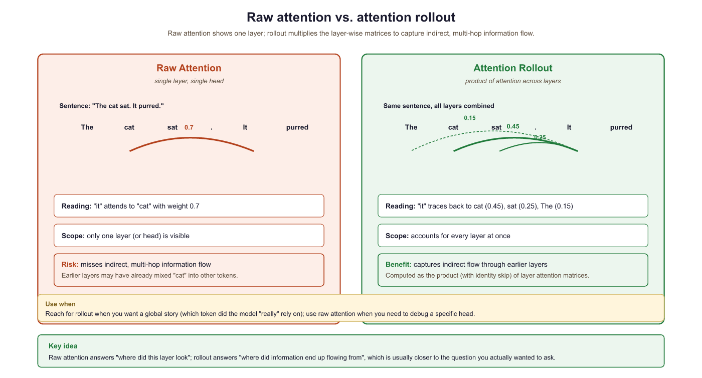
Raw attention weights from a single layer show direct token-to-token attention. But information flows through multiple layers, so a token at position 5 might influence position 10 indirectly by first attending to position 7, which then attends to position 10. Attention rollout (Abnar and Zuidema, 2020) accounts for this multi-hop information flow by multiplying attention matrices across layers. Figure 10.4.1 compares raw attention with attention rollout on the same input. Code Fragment 10.4.1a shows this approach in practice.
The following implementation computes attention rollout by multiplying attention matrices across all layers, accounting for softmax at each step.
Code Fragment 10.4.1c visualizes attention patterns.
# Attention Rollout Implementation
import torch
import numpy as np
def attention_rollout(
    attentions,
    head_fusion="mean",
    discard_ratio=0.0,
    ):
    """
                                                                                                                                                                                                                                                                                                                                                                                                                                                                                                                                                                                                                                                                                                                                                                                                                                    Compute attention rollout across all layers.
    Args:
    attentions: tuple of attention tensors, one per layer
    Each has shape (batch, num_heads, seq_len, seq_len)
    head_fusion: how to combine heads ("mean", "max", "min")
    discard_ratio: fraction of lowest attention weights to zero out
    Returns:
    rollout: (seq_len, seq_len) matrix of accumulated attention
    """
    num_layers = len(attentions)
    seq_len = attentions[0].shape[-1]
    # Start with identity (each token attends to itself)
    rollout = torch.eye(seq_len)
    for layer_idx in range(num_layers):
        attn = attentions[layer_idx].squeeze(0) # (heads, seq, seq)
        # Fuse attention heads
        if head_fusion == "mean":
            attn_fused = attn.mean(dim=0)
        elif head_fusion == "max":
            attn_fused = attn.max(dim=0).values
        elif head_fusion == "min":
            attn_fused = attn.min(dim=0).values
            # Optionally discard low-attention connections
            if discard_ratio > 0:
                flat = attn_fused.flatten()
                threshold = flat.quantile(discard_ratio)
                attn_fused = attn_fused * (attn_fused >= threshold)
                # Re-normalize rows
                attn_fused = attn_fused / attn_fused.sum(dim=-1, keepdim=True)
                # Add residual connection (identity)
                attn_with_residual = 0.5 * attn_fused + 0.5 * torch.eye(seq_len)
                # Multiply with cumulative rollout
                rollout = attn_with_residual @ rollout
                return rollout
                    # Usage
from transformers import AutoModelForCausalLM, AutoTokenizer
model = AutoModelForCausalLM.from_pretrained("gpt2", output_attentions=True)
tokenizer = AutoTokenizer.from_pretrained("gpt2")
text = "The cat sat on the mat because it was very tired"
inputs = tokenizer(text, return_tensors="pt")
outputs = model(**inputs)
rollout = attention_rollout(outputs.attentions)
tokens = tokenizer.convert_ids_to_tokens(inputs["input_ids"][0])
# Show which tokens "it" (position 7) attends to after rollout
it_idx = tokens.index("it") if "it" in tokens else 7
print(f"Attention rollout from '{tokens[it_idx]}':")
for i, (token, score) in enumerate(zip(tokens, rollout[it_idx])):
    bar = "#" * int(score.item() * 40)
print(f" {token:10s} {bar} ({score.item():.3f})")# Attention rollout: combine attention maps across all layers into a single
# matrix that approximates how information flows from input tokens to outputs.
# Reference: Abnar & Zuidema, "Quantifying Attention Flow in Transformers" (2020).
import torch
def attention_rollout(attentions: list[torch.Tensor],
discard_ratio: float = 0.0) -> torch.Tensor:
"""attentions: list of L tensors of shape (n_heads, seq_len, seq_len),
one per Transformer layer. Returns a (seq_len, seq_len) rollout matrix
where entry [i, j] approximates how much token j contributed to token i
at the top of the network."""
seq_len = attentions[0].size(-1)
result = torch.eye(seq_len)
for attn in attentions:
# Average across heads, add identity to model the residual stream,
# then renormalize so each row sums to 1.
head_mean = attn.mean(dim=0)
if discard_ratio > 0:
flat = head_mean.view(-1)
k = int(flat.numel() * discard_ratio)
threshold = flat.kthvalue(k).values
head_mean = torch.where(head_mean < threshold, torch.zeros_like(head_mean), head_mean)
aug = head_mean + torch.eye(seq_len)
aug = aug / aug.sum(dim=-1, keepdim=True)
result = aug @ result
return result
# Usage with a HuggingFace model that returns attentions:
# outputs = model(input_ids, output_attentions=True)
# attentions = [a[0] for a in outputs.attentions] # drop batch dim
# rollout = attention_rollout(attentions)
# influences = rollout[-1] # how much each input token contributed to the last positionThe implementation above builds attention rollout from scratch for pedagogical clarity. In production, use BertViz (install: pip install bertviz), which provides interactive attention visualizations at the head, model, and neuron levels (see Code Fragment 10.4.3 below).
# Production equivalent using BertViz
from bertviz import model_view, head_view
from transformers import AutoModel, AutoTokenizer
model = AutoModel.from_pretrained("gpt2", output_attentions=True)
tokenizer = AutoTokenizer.from_pretrained("gpt2")
inputs = tokenizer("The cat sat on the mat", return_tensors="pt")
outputs = model(**inputs)
head_view(outputs.attentions, tokenizer.convert_ids_to_tokens(inputs["input_ids"][0]))# Quick comparison: same task in TransformerLens vs nnsight vs nnterp
# === TransformerLens: full hook access, custom API ===
from transformer_lens import HookedTransformer
tl_model = HookedTransformer.from_pretrained("gpt2-small")
logits, cache = tl_model.run_with_cache("The cat sat on")
# Access any intermediate activation:
layer5_resid = cache["blocks.5.hook_resid_post"] # (1, seq, d_model)
# === nnsight: wrap any PyTorch model, proxy API ===
from nnsight import LanguageModel
nn_model = LanguageModel("gpt2", device_map="auto")
with nn_model.trace("The cat sat on") as tracer:
layer5_out = nn_model.transformer.h[5].output[0].save()
# Access saved activation after trace:
layer5_resid_nn = layer5_out.value # same shape
# === nnterp: lightweight, Hugging Face native ===
from nnterp import load_model, logit_lens
model, tokenizer = load_model("gpt2")
# Built-in logit lens with one call:
layer_predictions = logit_lens(model, tokenizer, "The cat sat on")
# Returns per-layer top predictions without manual unembeddingFor gradient-based attribution methods, see also Inseq (install: pip install inseq).
Attention rollout and the logit lens reveal where the model looks and what it predicts at each layer. But neither method tells us which attended tokens actually matter for the final output. To answer that question, we need to incorporate gradient information.
10.4.3 Gradient-Weighted Attention
Gradient-weighted attention (also called Attention × Gradient) combines attention weights with gradient information. The intuition is that attention tells us where the model looks, while gradients tell us how sensitive the output is to what the model finds there. Multiplying these signals highlights tokens that the model both attends to and that actually influence the prediction. Code Fragment 10.4.5 shows this approach in practice.
Code Fragment 10.4.5a combines attention weights with gradient information, highlighting tokens that both receive high attention and significantly influence the output.
# Gradient-Weighted Attention
import torch
def gradient_weighted_attention(
    model,
    tokenizer,
    text,
    target_pos=-1,
    ):
    """
    Compute gradient-weighted attention for each layer and head.
    Returns attention weights scaled by the gradient of the output
    with respect to the attention weights themselves.
    """
    model.eval()
    inputs = tokenizer(text, return_tensors="pt")
    tokens = tokenizer.convert_ids_to_tokens(inputs["input_ids"][0])
    # Forward pass with attention outputs
    outputs = model(**inputs, output_attentions=True)
    attentions = outputs.attentions # tuple of (1, heads, seq, seq)
    # Get the predicted token logit
    logits = outputs.logits[0, target_pos]
    predicted_token_id = logits.argmax()
    target_logit = logits[predicted_token_id]
    # Compute gradient of target logit w.r.t. each attention matrix
    grad_weighted = []
    for layer_attn in attentions:
        if layer_attn.requires_grad:
            grad = torch.autograd.grad(
                target_logit, layer_attn, retain_graph=True
                )[0]
            # Element-wise multiply: attention * gradient
            weighted = (layer_attn * grad).squeeze(0)
            # Average over heads
            weighted = weighted.mean(dim=0).detach()
            grad_weighted.append(weighted)
            # Stack and average across layers
            all_layers = torch.stack(grad_weighted) # (layers, seq, seq)
            combined = all_layers.mean(dim=0) # (seq, seq)
            return combined, tokens
            # Alternative: enable gradients for attention
            # Need to use hooks to capture attention with grad enabled
    def compute_attention_gradient_attribution(model, tokenizer, text):
        """Simpler approach using hooks to capture attention gradients."""
        attention_grads = {}
    def save_attention_grad(name):
        def hook(module, grad_input, grad_output):
            attention_grads[name] = grad_output[0].detach()
            return hook
            # Register backward hooks on attention layers
            hooks = []
            for i, layer in enumerate(model.transformer.h):
                h = layer.attn.register_full_backward_hook(
                    save_attention_grad(f"layer_{i}")
                    )
                hooks.append(h)
                # Forward + backward
                inputs = tokenizer(text, return_tensors="pt")
                outputs = model(**inputs, output_attentions=True)
                target = outputs.logits[0, -1].max()
                target.backward()
                # Clean up hooks
                for h in hooks:
                    h.remove()
return attention_grads10.4.4 Layer-wise Relevance Propagation (LRP)
Layer-wise Relevance Propagation redistributes the model's output score backward through the network, assigning a relevance value to each neuron at each layer. At the input layer, these relevance values become token-level attributions. LRP satisfies a conservation property: the total relevance at each layer equals the output score, ensuring nothing is lost or created during propagation.
LRP propagates relevance backward using a rule that distributes relevance proportionally to the contribution of each input. For a linear layer y = Wx + b, the relevance assigned to input x_i is proportional to how much x_i contributed to each output y_j, weighted by the relevance of y_j. The specific propagation rule (LRP-0, LRP-ε, LRP-γ) determines how to handle numerical stability and positive vs. negative contributions.
Who: Compliance team at a fintech lender using LLMs to draft loan decision explanations
Situation: Regulators required the company to explain why each loan application was approved or denied (a key concern in production safety and ethics), and the LLM-generated explanations needed to accurately reflect the model's actual reasoning.
Problem: The LLM produced plausible-sounding explanations, but there was no guarantee that the cited factors (income, credit history) actually drove the prediction. Regulators flagged this as a "post-hoc rationalization" risk.
Dilemma: Attention weights were easy to extract but unreliable as explanations (attention does not equal attribution). Full Integrated Gradients were accurate but too slow for real-time decision explanations.
Decision: They implemented Layer-wise Relevance Propagation (LRP), which provided faithful token-level attributions faster than Integrated Gradients while satisfying the conservation property required for audit trails.
How: LRP propagated relevance backward from the decision token through all transformer layers, producing a per-input-token relevance score. The top-5 relevant input features were extracted and mapped to human-readable factors.
Result: LRP-based explanations aligned with the actual decision drivers 91% of the time (verified by feature ablation tests), compared to 64% for attention-based explanations. Processing time was 120ms per application, meeting the real-time requirement. The regulator accepted LRP attributions as compliant explanations.
Lesson: For regulated applications requiring faithful explanations, LRP provides a principled middle ground between unreliable attention visualization and computationally expensive gradient integration. Code Fragment 10.4.6 shows this approach in practice.
The following simplified LRP implementation propagates relevance backward through linear layers using the epsilon rule for numerical stability.
# Layer-wise Relevance Propagation for Transformers (simplified)
import torch
import torch.nn as nn
class TransformerLRP:
    """Simplified LRP for transformer models."""
    def __init__(self, model, epsilon=1e-6):
        self.model = model
        self.epsilon = epsilon
        self.activations = {}
    def register_hooks(self):
        """Register forward hooks to capture activations."""
        self.hooks = []
        for name, module in self.model.named_modules():
            if isinstance(module, nn.Linear):
                h = module.register_forward_hook(
                    self._save_activation(name)
                    )
                self.hooks.append(h)
    def _save_activation(self, name):
        def hook(module, input, output):
            self.activations[name] = {
                "input": input[0].detach(),
                "output": output.detach(),
                "weight": module.weight.detach(),
                }
            return hook
        def propagate_linear(self, relevance, layer_name):
            """LRP-epsilon rule for a linear layer."""
            act = self.activations[layer_name]
            z = act["input"] @ act["weight"].T # pre-activation
            z = z + self.epsilon * z.sign() # stabilize
            s = relevance / z
            c = s @ act["weight"]
            relevance_input = act["input"] * c
            return relevance_input
        def attribute(self, text, tokenizer):
            """Compute LRP attribution for input tokens."""
            self.register_hooks()
            inputs = tokenizer(text, return_tensors="pt")
            with torch.no_grad():
                outputs = self.model(**inputs)
                # Start with the output logits as initial relevance
                logits = outputs.logits[0, -1]
                relevance = torch.zeros_like(logits)
                relevance[logits.argmax()] = logits.max()
                # Propagate backward through the network
                # (simplified: in practice, need to handle attention specially)
                for name in reversed(list(self.activations.keys())):
                    if name.startswith("lm_head") or "mlp" in name:
                        relevance = self.propagate_linear(relevance, name)
                        # Clean up
                        for h in self.hooks:
                            h.remove()
return relevance10.4.5 Perturbation-Based Explanations
Perturbation methods explain predictions by measuring how the output changes when parts of the input are modified or removed. Unlike gradient-based methods (which measure local sensitivity), perturbation methods measure actual counterfactual impact: what would the model predict if this token were absent? Code Fragment 10.5.1 shows this approach in practice.
The following implementations measure token importance through direct removal: leave-one-out tests individual tokens, while sliding window occlusion captures multi-token patterns.
# Perturbation-based attribution methods
import torch
import numpy as np
def leave_one_out_attribution(model, tokenizer, text):
    """
    Measure each token's importance by removing it and
    observing the change in prediction confidence.
    """
    inputs = tokenizer(text, return_tensors="pt")
    tokens = tokenizer.convert_ids_to_tokens(inputs["input_ids"][0])
    # Get baseline prediction
    with torch.no_grad():
        baseline_logits = model(**inputs).logits[0, -1]
        baseline_probs = torch.softmax(baseline_logits, dim=-1)
        predicted_id = baseline_probs.argmax()
        baseline_prob = baseline_probs[predicted_id].item()
        # Remove each token and measure impact
        attributions = []
        for i in range(len(tokens)):
            # Create input with token i replaced by padding/mask
            perturbed_ids = inputs["input_ids"].clone()
            perturbed_ids[0, i] = tokenizer.pad_token_id or 0
            with torch.no_grad():
                perturbed_logits = model(perturbed_ids).logits[0, -1]
                perturbed_prob = torch.softmax(perturbed_logits, dim=-1)[predicted_id].item()
                # Attribution = drop in probability when token is removed
                attribution = baseline_prob - perturbed_prob
                attributions.append(attribution)
                return np.array(attributions), tokens
    def sliding_window_occlusion(
        model, tokenizer, text, window_size=3
        ):
        """
        Occlude a sliding window of tokens to find important regions.
        More robust than single-token removal for capturing multi-token patterns.
        """
        inputs = tokenizer(text, return_tensors="pt")
        tokens = tokenizer.convert_ids_to_tokens(inputs["input_ids"][0])
        seq_len = len(tokens)
        with torch.no_grad():
            baseline_logits = model(**inputs).logits[0, -1]
            predicted_id = baseline_logits.argmax()
            baseline_score = baseline_logits[predicted_id].item()
            region_scores = []
            for start in range(seq_len - window_size + 1):
                perturbed_ids = inputs["input_ids"].clone()
                for j in range(start, start + window_size):
                    perturbed_ids[0, j] = tokenizer.pad_token_id or 0
                    with torch.no_grad():
                        perturbed_logits = model(perturbed_ids).logits[0, -1]
                        score = perturbed_logits[predicted_id].item()
                        impact = baseline_score - score
                        region_scores.append({
                            "start": start,
                            "end": start + window_size,
                            "tokens": tokens[start:start + window_size],
                            "impact": impact,
                            })
                        # Sort by impact
                        region_scores.sort(key=lambda x: x["impact"], reverse=True)
return region_scoresPerturbation methods have a fundamental limitation: removing a token creates an out-of-distribution input. The model was never trained on inputs with random tokens in the middle of coherent text, so its behavior on perturbed inputs may not reflect what it would do if the token were genuinely absent. This is sometimes called the "off-manifold" problem. Methods like SHAP (Section 10.3) partially address this by marginalizing over replacements rather than using a fixed perturbation.
10.4.6 Comparing Explanation Methods
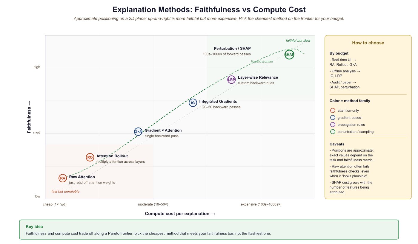
Different explanation methods can produce substantially different attributions for the same prediction. Choosing the right method requires understanding what each method measures and what properties matter for your use case. Figure 10.4.2a positions the major methods on a faithfulness versus computational cost axis.
| Method | What It Measures | Strengths | Weaknesses |
|---|---|---|---|
| Raw attention | Where the model "looks" | Fast, intuitive, no extra computation | Not faithful; ignores values and MLPs |
| Attention rollout | Multi-layer information flow | Captures indirect paths across layers | Still ignores value vectors and MLPs |
| Grad x Attention | Gradient-weighted attention flow | Combines where model looks with sensitivity | Gradients can be noisy, local approximation |
| Integrated Gradients | Path-integrated sensitivity | Axiom-satisfying, theoretically grounded | Baseline choice matters, can be expensive |
| LRP | Backward relevance propagation | Conservation property, layer-specific | Complex to implement for attention layers |
| Perturbation/SHAP | Counterfactual impact of removal | Most direct measure of importance | Off-manifold problem, very expensive |
Recent work suggests that no attribution method consistently outperforms others across all evaluation metrics. The best choice depends on the application: for quick debugging, raw attention or attention rollout provides fast insight; for regulatory compliance requiring faithful explanations, Integrated Gradients or SHAP is more appropriate; for mechanistic understanding, activation patching (Section 10.2) provides the strongest causal evidence. Code Fragment 10.5.2 shows this approach in practice.
Code Fragment 10.5.2a runs multiple attribution methods on the same input and computes rank correlations to measure agreement between them.
# Unified comparison framework for explanation methods
import torch
import numpy as np
from typing import Dict, Callable, List
def compare_attribution_methods(
    model,
    tokenizer,
    text: str,
    methods: Dict[str, Callable],
    ) -> Dict[str, np.ndarray]:
    """
    Run multiple attribution methods on the same input
    and compare their outputs.
    """
    results = {}
    tokens = tokenizer.convert_ids_to_tokens(
        tokenizer(text, return_tensors="pt")["input_ids"][0]
        )
    for name, method_fn in methods.items():
        attributions = method_fn(model, tokenizer, text)
        # Normalize to [0, 1] for comparison
        attr_min = attributions.min()
        attr_max = attributions.max()
        if attr_max > attr_min:
            normalized = (attributions - attr_min) / (attr_max - attr_min)
        else:
            normalized = np.zeros_like(attributions)
            results[name] = normalized
            # Compute agreement metrics
            method_names = list(results.keys())
            print(f"Attribution comparison for: '{text}'")
            print(f"Predicted next token: {get_prediction(model, tokenizer, text)}")
            print()
            # Rank correlation between methods
            from scipy.stats import spearmanr
            print("Spearman rank correlations:")
            for i, name_a in enumerate(method_names):
                for name_b in method_names[i+1:]:
                    corr, pval = spearmanr(results[name_a], results[name_b])
                    print(f" {name_a} vs {name_b}: rho={corr:.3f} (p={pval:.3f})")
                    # Top-3 tokens per method
                    print("\nTop-3 most important tokens per method:")
                    for name, attrs in results.items():
                        top_3 = np.argsort(attrs)[-3:][::-1]
                        top_tokens = [(tokens[i], attrs[i]) for i in top_3]
                        top_str = ", ".join(f"'{t}' ({s:.2f})" for t, s in top_tokens)
                        print(f" {name:20s}: {top_str}")
                        return results
                        # Run comparison
                        methods = {
                            "raw_attention": lambda m, t, x: extract_raw_attention(m, t, x),
                            "rollout": lambda m, t, x: compute_rollout(m, t, x),
                            "integrated_gradients": lambda m, t, x: integrated_gradients(m, t, x)[0],
                            "leave_one_out": lambda m, t, x: leave_one_out_attribution(m, t, x)[0],
                            }
                        results = compare_attribution_methods(
                            model, tokenizer,
                            "The Eiffel Tower is located in the city of",
                            methods
)When different attribution methods disagree about which tokens are important, this is informative rather than problematic. Disagreement typically occurs because the methods measure different things: attention rollout captures information flow regardless of what is done with it, gradients measure local sensitivity, and perturbation methods measure actual counterfactual impact. Using multiple methods together provides a more complete picture than any single method alone.
- Different explanation methods measure fundamentally different things: where the model looks (attention), local sensitivity (gradients), path-integrated contribution (IG), backward relevance (LRP), and counterfactual impact (perturbation).
- Attention rollout accounts for multi-layer information flow by multiplying attention matrices across layers, capturing indirect paths that raw attention misses.
- Gradient-weighted attention combines the "where" of attention with the "how much it matters" of gradients, filtering out uninformative attention patterns.
- Perturbation-based methods provide the most direct measure of token importance but suffer from the off-manifold problem when creating unnatural inputs.
- No single explanation method dominates across all use cases. Choose based on your needs: fast insight (attention), theoretical guarantees (IG), or counterfactual reasoning (perturbation).
Show Answer
Show Answer
Show Answer
Show Answer
What Comes Next
The next section, Section 10.5: Interpretability Tooling, Evaluation, and LLM-Assisted Explanation, completes the explanation toolkit by surveying production XAI libraries (Captum, LIME, BertViz), faithfulness and plausibility evaluation metrics, and the new wave of LLM-assisted explanation workflows.