"A method without a tool is a lecture; a tool without a method is a toy. Interpretability needs both."
Probe, Tool-Smith AI Agent
Section 10.4 introduced the attribution methods (attention rollout, gradient-weighted attention, LRP, perturbation, integrated gradients). This continuation answers three operational questions: which open-source tools run those methods at scale, how to evaluate the explanations they produce (faithfulness vs. plausibility), and how LLMs themselves are becoming explanation assistants that narrate the outputs of other models. Together these three layers close the loop from "I have a method" to "I have an explanation I can ship and audit".
Prerequisites
This section continues from Section 10.4: Explaining Transformers, which introduced the core attribution methods that the tools below operationalize. Familiarity with attention analysis and probing from Section 10.1 is also assumed.
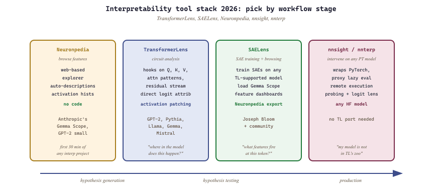
10.5.1 Interpretability Tools Ecosystem (2025)
The interpretability research community has built a rich ecosystem of open-source tools over the past three years. Choosing the right tool depends on your goal: are you doing mechanistic circuit analysis, exploring SAE features, or building a production explanation pipeline? This section surveys the major tools and helps you match tools to use cases.
A neurologist who suspects a stroke does not lecture the patient about brain anatomy; she orders a scan and reads what lights up. Interpretability tooling for LLMs is the same workflow with different equipment: activation patching is the scan, sparse autoencoders are the contrast dye, and an LLM-as-explainer is a junior radiologist drafting the report. The patient cannot tell you what they were thinking; the scan can.
Why does the tooling matter? Interpretability research is only as reproducible and accessible as its tooling. A brilliant mechanistic finding that requires custom infrastructure to replicate has limited impact. The tools listed below have lowered the barrier to entry, enabling researchers and practitioners to run experiments that previously required months of infrastructure work.
| Tool | Primary Use | Key Features | Best For |
|---|---|---|---|
| TransformerLens | Mechanistic interpretability | Full hook access at every sub-computation (Q, K, V, attention patterns, residual stream); built-in caching; direct logit attribution | Detailed circuit analysis on supported models (GPT-2, Pythia, Llama, Gemma, Mistral) |
| SAELens | SAE training and analysis | Train SAEs on any TransformerLens model; load pretrained Gemma Scope SAEs; feature dashboard generation; integration with Neuronpedia | Training custom SAEs, loading Gemma Scope, feature-level analysis |
| Neuronpedia | Feature browsing and search | Web-based feature explorer; auto-generated descriptions; activation histograms; community annotations; cross-model comparisons | Non-code exploration of SAE features; sharing and discussing findings |
| nnsight | Model intervention | Wraps any PyTorch primitives model; proxy-based lazy evaluation; remote execution support; familiar PyTorch API | Quick experiments on any architecture, including models not supported by TransformerLens |
| nnterp | Neural network interpretation | Probing, logit lens, representation analysis; lightweight API; works with Hugging Face models directly | Probing experiments and logit lens analysis without TransformerLens overhead |
Tool selection depends on your interpretability workflow stage. For hypothesis generation (browsing features, visualizing attention), start with Neuronpedia and standard Hugging Face tools. For hypothesis testing (activation patching, circuit tracing), use TransformerLens or nnsight. For SAE training and feature analysis, use SAELens. For lightweight probing and logit lens experiments, nnterp provides a lower-overhead alternative. Many researchers combine multiple tools: SAELens for training SAEs, TransformerLens for circuit analysis, and Neuronpedia for browsing results.
# Same task in three frameworks: extract activations from layer 5 of GPT-2.
# Each library trades off ease of use for control over the model internals.

# (A) Plain HuggingFace transformers + a forward hook
from transformers import AutoModelForCausalLM, AutoTokenizer
import torch
tok = AutoTokenizer.from_pretrained("gpt2")
model_hf = AutoModelForCausalLM.from_pretrained("gpt2")
acts_hf = {}
def hook(module, inputs, output):
    acts_hf["layer5"] = output[0]
model_hf.transformer.h[5].register_forward_hook(hook)
model_hf(**tok("The Eiffel Tower is in", return_tensors="pt"))
print("HF activations:", acts_hf["layer5"].shape)

# (B) nnsight: pause execution mid-forward and pull values declaratively
from nnsight import LanguageModel
model_ns = LanguageModel("gpt2")
with model_ns.trace("The Eiffel Tower is in"):
    layer5_acts = model_ns.transformer.h[5].output[0].save()
print("nnsight activations:", layer5_acts.shape)

# (C) transformer_lens: built-in HookedTransformer with named hook points
from transformer_lens import HookedTransformer
model_tl = HookedTransformer.from_pretrained("gpt2")
_, cache = model_tl.run_with_cache("The Eiffel Tower is in")
print("transformer_lens activations:", cache["blocks.5.hook_resid_post"].shape)
# All three return the same tensor; the differences are in API ergonomics.10.5.1.1 Production XAI Libraries: Captum, LIME, and BertViz
The tools above (TransformerLens, SAELens, nnsight) serve the mechanistic interpretability community, where the goal is understanding internal model computations. A complementary set of tools addresses the production explainability problem: generating human-readable explanations of individual predictions for end users, auditors, or regulatory compliance. These libraries treat the model as a function (sometimes a black box) and explain its input-output behavior rather than its internal circuits.
Captum: Meta's Attribution Toolkit
Captum is Meta's comprehensive model interpretability library for PyTorch. It implements over a dozen attribution methods under a unified API, making it straightforward to compare different explanation approaches on the same prediction. For transformer models, the most commonly used methods are Layer Integrated Gradients (attributing to the embedding layer), Layer Gradient x Activation, and Layer Conductance (which measures the importance of individual neurons in a specific layer).
Captum's strength is its breadth: it covers gradient-based methods (Integrated Gradients, DeepLift, GradientSHAP), perturbation-based methods (Feature Ablation, Shapley Value Sampling, LIME via the Lime wrapper), and layer-level methods (Layer Conductance, Internal Influence). This means you can compare multiple explanation strategies on the same model without switching libraries.
The full Captum attribution catalog spans roughly twenty methods, organized into three families: primary attribution (Integrated Gradients, Saliency, DeepLift, DeepLiftShap, GradientShap, InputXGradient, GuidedBackprop, GuidedGradCam, Deconvolution, Feature Ablation, Feature Permutation, Occlusion, Shapley Value Sampling, Lime, KernelShap), layer attribution (LayerConductance, LayerIntegratedGradients, LayerGradientXActivation, LayerGradCam, LayerDeepLift, LayerActivation, InternalInfluence), and neuron attribution (NeuronConductance, NeuronGradient, NeuronIntegratedGradients). Most methods share the same .attribute(inputs, ...) API, so swapping methods is usually a one-line change. The official Captum site keeps a visual algorithm zoo chart that maps each method to its theoretical family and recommended use case; consult it before picking a method for a novel modality.
Captum on image classification (vision)
Captum is not text-only. Applied to an image classifier (a ResNet-50 or ViT, for example), Layer Integrated Gradients produces a per-pixel saliency map for any chosen target class. The recipe is exactly the same as the text case: wrap the model's forward pass, choose a baseline (typically a zero or blurred image), pick a target class index, and call .attribute(). Captum then returns a tensor of the same shape as the input image, and captum.attr.visualization.visualize_image_attr overlays the saliency map on the original image. The two-line summary is:
from captum.attr import IntegratedGradients, visualization as viz
ig = IntegratedGradients(resnet50)
attr = ig.attribute(image_tensor, target=predicted_class, n_steps=50)
viz.visualize_image_attr(attr.squeeze().cpu().permute(1,2,0).numpy(),
original_image, method="heat_map", sign="positive")[PAD] tokens) and the visualization helper change. Useful for sanity-checking whether the model relies on object features or shortcuts like watermarks and backgrounds.# Comprehensive Captum attribution for a transformer classifier
import torch
from transformers import AutoModelForSequenceClassification, AutoTokenizer
from captum.attr import (
LayerIntegratedGradients,
LayerGradientXActivation,
LayerConductance,
visualization as viz,
)
model_name = "distilbert-base-uncased-finetuned-sst-2-english"
model = AutoModelForSequenceClassification.from_pretrained(model_name)
tokenizer = AutoTokenizer.from_pretrained(model_name)
model.eval()
text = "The movie was surprisingly entertaining despite a weak script"
inputs = tokenizer(text, return_tensors="pt")
input_ids = inputs["input_ids"]
baseline_ids = torch.zeros_like(input_ids) # PAD token baseline
# Wrap the forward function for Captum
def forward_func(input_ids):
outputs = model(input_ids)
return outputs.logits[:, 1] # positive sentiment logit
# Method 1: Layer Integrated Gradients (most common for transformers)
lig = LayerIntegratedGradients(forward_func, model.distilbert.embeddings)
attrs_ig, delta = lig.attribute(
input_ids, baselines=baseline_ids,
n_steps=50, return_convergence_delta=True,
)
# Convergence delta should be small (< 0.05); large values indicate
# that n_steps is too low for accurate integration.
# Method 2: Gradient x Activation (faster, less theoretically grounded)
lga = LayerGradientXActivation(forward_func, model.distilbert.embeddings)
attrs_gxa = lga.attribute(input_ids)
# Method 3: Layer Conductance (neuron-level importance in a specific layer)
lc = LayerConductance(forward_func, model.distilbert.transformer.layer[3])
attrs_cond = lc.attribute(input_ids, baselines=baseline_ids, n_steps=20)
# Summarize per-token attributions
tokens = tokenizer.convert_ids_to_tokens(input_ids[0])
attrs_sum = attrs_ig.sum(dim=-1).squeeze(0).detach().numpy()
print("Integrated Gradients attribution per token:")
for tok, score in zip(tokens, attrs_sum):
bar = "#" * int(min(abs(score) * 10, 40))
sign = "+" if score > 0 else "-"
print(f" {tok:20s} {sign}{bar:40s} {score:+.4f}")LIME for Language Models
LIME (Local Interpretable Model-agnostic Explanations) explains individual predictions by fitting a simple interpretable model (typically a sparse linear model) to the behavior of the complex model in the neighborhood of a specific input. For text, LIME works by randomly removing words from the input, observing how the model's prediction changes, and fitting a linear model that approximates the local decision boundary.
LIME's key advantage is that it is entirely model-agnostic: it treats the model as a black box and requires only the ability to call the model's prediction function. This makes it applicable to API-based LLMs where you have no access to gradients or internal activations. The tradeoff is that LIME's perturbation strategy (removing tokens) can create out-of-distribution inputs that a language model has never seen during training, potentially producing misleading attributions.
import torch
# LIME explanation for a text classifier (model-agnostic)
from lime.lime_text import LimeTextExplainer
import numpy as np
# Works with any model that returns class probabilities
def predict_proba(texts):
    """Prediction function that LIME will call repeatedly."""
    results = []
    for text in texts:
        inputs = tokenizer(text, return_tensors="pt",
            truncation=True, max_length=512)
        with torch.no_grad():
            logits = model(**inputs).logits[0]
            probs = torch.softmax(logits, dim=-1).numpy()
            results.append(probs)
            return np.array(results)
        explainer = LimeTextExplainer(class_names=["negative", "positive"])
        text = "The movie was surprisingly entertaining despite a weak script"
        explanation = explainer.explain_instance(
            text,
            predict_proba,
            num_features=10, # top 10 most important words
            num_samples=1000, # number of perturbations to generate
            )
        # Display word-level importance
        print("LIME feature importance (positive sentiment):")
        for word, weight in explanation.as_list():
            direction = "+" if weight > 0 else "-"
            bar = "#" * int(abs(weight) * 50)
            print(f" {word:20s} {direction}{bar} ({weight:+.4f})")
            # LIME also provides HTML visualization:
            # explanation.save_to_file("lime_explanation.html")
            # For API-based LLMs (no gradient access), LIME is often the only option.
            # Replace predict_proba with an API call wrapper:
            #
            # def predict_proba_api(texts):
            # results = []
            # for text in texts:
            # response = client.chat.completions.create(
            # model="gpt-4o-mini",
            # messages=[{"role": "user", "content": f"Classify: {text}"}],
            # logprobs=True,
            # )
            # # Extract probabilities from logprobs
            # results.append(parse_logprobs(response))
            # return np.array(results)
BertViz: Interactive Attention Visualization
BertViz provides interactive, browser-based visualizations of attention patterns across all layers and heads of a transformer model. It offers three visualization modes: the head view (attention from a single head as lines connecting tokens), the model view (all heads across all layers in a compact overview), and the neuron view (how individual neurons in Q, K, V contribute to attention). BertViz works in Jupyter notebooks and supports BERT, GPT-2, RoBERTa, XLNet, and other Hugging Face models.
While Section 10.1 covered attention visualization from scratch, BertViz is the production tool for this task. It is particularly useful for qualitative exploration: scanning attention patterns across layers to identify which heads attend to syntactic structure, which heads focus on positional patterns, and which heads appear to implement specific linguistic functions like coreference resolution or subject-verb agreement.
# BertViz: interactive attention visualization in Jupyter
# pip install bertviz
from bertviz import model_view, head_view, neuron_view
from transformers import AutoModel, AutoTokenizer
model = AutoModel.from_pretrained("bert-base-uncased",
    output_attentions=True)
tokenizer = AutoTokenizer.from_pretrained("bert-base-uncased")
text = "The bank raised interest rates after the financial crisis"
inputs = tokenizer(text, return_tensors="pt")
outputs = model(**inputs)
attention = outputs.attentions # tuple of (batch, heads, seq, seq) per layer
tokens = tokenizer.convert_ids_to_tokens(inputs["input_ids"][0])
# Model view: compact overview of all layers and heads
model_view(attention, tokens)
# Head view: detailed view for a specific layer
head_view(attention, tokens, layer=6, heads=[0, 3, 7])
# Neuron view: see Q/K/V contributions (requires special model loading)
# neuron_view(model, tokenizer, text, layer=6, head=3)
# Practical usage pattern: identify interesting heads, then investigate
# with probing classifiers (Section 10.1) or activation patching
# (Section 10.2) to confirm functional roles.The choice between XAI libraries depends on three factors: model access (do you have gradient access, or only API access?), audience (researchers, engineers, or non-technical stakeholders?), and goal (debugging a specific failure, or systematic audit for compliance?). If you have full model access and need theoretically grounded attributions, use Captum with Integrated Gradients. If you only have API access, use LIME with a prediction wrapper. If you are exploring attention patterns during model development, use BertViz for interactive visualization. For mechanistic circuit analysis during research, use TransformerLens. For regulatory audits requiring feature-level explanations, combine Captum (for attributions) with SHAP (for Shapley-value guarantees from Section 10.3).
| Scenario | Model Access | Recommended Tool(s) | Output |
|---|---|---|---|
| Debug misclassification in production | Full (local model) | Captum (Integrated Gradients) | Per-token attribution scores |
| Explain API-based LLM predictions | API only | LIME | Word-level importance, local linear model |
| Explore attention during development | Full | BertViz | Interactive attention heatmaps |
| Regulatory compliance audit | Full | SHAP + Captum | Shapley values with theoretical guarantees |
| Research: understand model circuits | Full | TransformerLens + SAELens | Activation patches, feature dashboards |
| Quick probing and logit lens | Full | nnterp | Per-layer predictions, probing accuracy |
| Non-technical stakeholder report | Any | LIME or Captum + custom visualization | Highlighted text, plain-language summaries |
10.5.2 Evaluation of Explanation Quality
How do we know if an explanation is "good"? Several metrics have been proposed to evaluate explanation quality, each capturing different desirable properties.
| Metric | What It Measures | How to Compute |
|---|---|---|
| Faithfulness (Sufficiency) | Can the top-k tokens reproduce the prediction? | Keep only top-k attributed tokens, measure prediction change |
| Faithfulness (Comprehensiveness) | Do the top-k tokens account for the prediction? | Remove top-k tokens, measure prediction drop |
| Plausibility | Do explanations match human intuition? | Compare attributions to human annotation of important words |
| Consistency | Do similar inputs get similar explanations? | Measure attribution similarity for paraphrased inputs |
| Sparsity | How concentrated is the attribution? | Entropy or Gini coefficient of attribution distribution |
Code Fragment 10.5.5 demonstrates this approach.
Code Fragment 10.5.5a evaluates whether the attributed tokens actually drive the prediction, using both sufficiency (keeping only top-k) and comprehensiveness (removing top-k) tests.
import numpy as np
import torch
# Faithfulness evaluation for attribution methods
def evaluate_faithfulness(
    model,
    tokenizer,
    text,
    attributions,
    k_values=[1, 3, 5],
    ):
    """
    Evaluate faithfulness of attributions using sufficiency and comprehensiveness.
    """
    inputs = tokenizer(text, return_tensors="pt")
    tokens = tokenizer.convert_ids_to_tokens(inputs["input_ids"][0])
    with torch.no_grad():
        baseline_logits = model(**inputs).logits[0, -1]
        predicted_id = baseline_logits.argmax()
        baseline_prob = torch.softmax(baseline_logits, dim=-1)[predicted_id].item()
        sorted_indices = np.argsort(attributions)[::-1]
        results = {}
        for k in k_values:
            top_k = sorted_indices[:k]
            # Sufficiency: keep only top-k tokens
            sufficient_ids = inputs["input_ids"].clone()
            mask = torch.ones(len(tokens), dtype=torch.bool)
            mask[list(top_k)] = False
            sufficient_ids[0, mask] = tokenizer.pad_token_id or 0
            with torch.no_grad():
                suf_logits = model(sufficient_ids).logits[0, -1]
                suf_prob = torch.softmax(suf_logits, dim=-1)[predicted_id].item()
                sufficiency = suf_prob / baseline_prob # closer to 1 = better
                # Comprehensiveness: remove top-k tokens
                comp_ids = inputs["input_ids"].clone()
                for idx in top_k:
                    comp_ids[0, idx] = tokenizer.pad_token_id or 0
                    with torch.no_grad():
                        comp_logits = model(comp_ids).logits[0, -1]
                        comp_prob = torch.softmax(comp_logits, dim=-1)[predicted_id].item()
                        comprehensiveness = 1 - (comp_prob / baseline_prob) # closer to 1 = better
                        results[f"k={k}"] = {
                            "sufficiency": sufficiency,
                            "comprehensiveness": comprehensiveness,
                            }
                        return results
10.5.3 LLMs as Interpretability Assistants
A surprising twist in the interpretability story is that LLMs themselves have become powerful tools for explaining other models. Instead of relying solely on numerical attribution scores or heatmaps, practitioners are using language models to generate natural language explanations of model behavior, produce counterfactual analyses, and even automate the labeling of internal model features discovered through mechanistic interpretability.
10.5.3.1 Natural Language Explanations of Predictions
Given a model's input, output, and attribution scores, an LLM can synthesize a human-readable explanation: "The model predicted negative sentiment primarily because of the phrase 'deeply disappointed,' which received the highest attribution score. The word 'excellent' in the second sentence pulled toward positive sentiment but was outweighed by the negative signals." This transforms opaque numerical outputs into narratives that stakeholders can understand and critique. The key advantage is accessibility: a product manager does not need to interpret a SHAP waterfall chart if an LLM can narrate the same information in plain language.
10.5.3.2 LLM-Generated Counterfactual Explanations
Counterfactual explanations answer the question "what would need to change for the prediction to be different?" An LLM can generate these by prompting it with the original input and prediction, then asking it to produce minimal modifications that would flip the outcome. For example: "The loan application was denied because the debt-to-income ratio of 45% exceeds the threshold. The prediction would change to approved if the monthly debt payments decreased from $2,700 to below $2,000, or if annual income increased from $72,000 to above $85,000." These explanations are actionable in ways that feature importance scores are not, and they satisfy regulatory requirements in domains like finance and healthcare where model decisions must be explainable.
10.5.3.3 Automated Model Card Generation
Model cards (Mitchell et al., 2019) document a model's intended use, performance characteristics, limitations, and ethical considerations. Writing them manually is tedious and often skipped. LLMs can automate this by analyzing a model's evaluation results, training data statistics, and configuration, then generating a structured model card that covers performance breakdowns by demographic group, known failure modes, and recommended use cases. While the generated card requires human review, it reduces the documentation burden from hours to minutes and ensures that no standard section is accidentally omitted.
10.5.3.4 Auto-Labeling SAE Features with LLMs
The sparse autoencoders (SAEs) discussed in Section 10.3 decompose model activations into thousands of interpretable features, but each feature needs a human-readable label to be useful. OpenAI's "Language models can explain neurons in language models" (Bills et al., 2023) pioneered the approach of using GPT-4 to automatically describe what each neuron computes by showing it the neuron's top-activating examples and asking for a natural language summary. Neuronpedia scales this approach to the features discovered by SAEs, using LLMs to auto-label features from Gemma Scope (covered earlier in Section 10.3) and other SAE analyses. The process works as follows: collect the top 20 text examples that maximally activate a given SAE feature, present them to an LLM with the prompt "What concept or pattern do these examples share?", and store the generated label alongside the feature. Human spot-checks verify label quality, and the community can propose corrections.
Using LLMs to explain other models creates a productive feedback loop: interpretability techniques surface internal features, LLMs label those features in natural language, and researchers use the labels to form hypotheses about model behavior that drive further investigation. The risk is circular reasoning; if the explaining LLM shares biases or blind spots with the model being explained, the generated labels may be plausible but misleading. Always validate LLM-generated explanations against ground truth or human judgment, especially for safety-critical applications.
10.5.3.5 Practical Workflow
A typical LLM-assisted interpretability workflow combines the techniques above. First, run standard attribution methods (Integrated Gradients, attention rollout) on a set of important predictions. Second, feed the attributions into an LLM to generate natural language explanations and counterfactuals. Third, use SAE feature analysis with LLM auto-labeling to identify higher-level circuits involved in the prediction. Fourth, compile the results into an auto-generated model card. This end-to-end pipeline makes interpretability accessible to teams that lack dedicated interpretability researchers, democratizing a practice that was previously confined to specialized labs.
The logit lens family of techniques (including the tuned lens and future lens) is revealing how transformer layers progressively refine predictions, providing a window into the computation happening across depth. Research on universal neurons and induction heads has identified recurring computational motifs that appear across different transformer architectures and training runs, suggesting fundamental building blocks of language model computation. An open frontier is using interpretability findings to design better architectures, closing the loop from understanding to engineering by building models whose internal computations are more transparent by construction.
- The interpretability toolkit divides into mechanistic tools (TransformerLens, SAELens, Neuronpedia, nnsight, nnterp) for circuit-level work and production XAI libraries (Captum, LIME, BertViz, SHAP) for shipping explanations.
- Pick the tool by access and audience: gradient access + research goal favors Captum/TransformerLens; API-only access forces you toward LIME; non-technical audiences are best served by LIME or Captum plus a custom visualization layer.
- Faithfulness (does the explanation reflect the model?) and plausibility (does it make sense to humans?) are distinct axes. Sufficiency and comprehensiveness operationalize faithfulness as concrete ablation tests.
- LLM-assisted interpretability turns numerical attributions into narratives, generates actionable counterfactuals, automates model cards, and labels SAE features. Treat LLM-generated explanations as drafts that need validation, not as ground truth.
- A modern interpretability workflow chains all three layers: methods produce attributions, tools run the methods at scale, and an explainer LLM packages the result for the audience that needs it.
Show Answer
Show Answer
Show Answer
Exercises
Feature visualization is well-developed for vision models (generating images that maximally activate a neuron). Why is the equivalent for LLMs more challenging, and what alternative approaches exist?
Answer Sketch
For vision models, you can optimize an input image via gradient ascent to maximize a neuron's activation, producing a human-interpretable image. For LLMs, the input is discrete tokens, so gradient ascent does not directly apply (you cannot have a 'fractional token'). Alternatives: (1) Dataset examples: find real text that maximally activates the feature (the approach used in the previous exercise). (2) Logit attribution: see which output tokens the feature promotes or suppresses. (3) Automated interpretability: use another LLM to describe what a feature responds to. (4) Optimization in embedding space followed by nearest-token projection (approximate but sometimes useful). Dataset examples are the most common approach because they show real-world contexts where the feature fires.
Representation engineering studies how high-level concepts (truthfulness, safety, emotion) are encoded as directions in a model's activation space. Explain the basic approach: how do you find the 'truthfulness direction'?
Answer Sketch
Create pairs of prompts designed to elicit truthful vs. untruthful model behavior (e.g., true statements vs. common misconceptions). Run both sets through the model and record activations at each layer. The 'truthfulness direction' is the vector that best separates truthful from untruthful activations (often found via PCA on the difference vectors). This direction can then be used to: (1) classify whether the model is being truthful on new inputs. (2) Steer the model toward truthfulness by adding the direction vector to activations during inference. The approach assumes that concepts are encoded as linear directions, which is approximately true for many high-level properties.
Some researchers argue that interpretability is necessary for safe AGI because behavioral testing alone cannot guarantee safety. Others argue that interpretability methods will always lag behind model complexity. Evaluate both positions and suggest a middle ground.
Answer Sketch
Pro-interpretability: behavioral testing only covers tested scenarios; a model could behave safely in known situations but dangerously in novel ones. Interpretability could identify dangerous internal representations (deception, power-seeking) before they manifest behaviorally. This is analogous to X-raying a machine rather than just watching it operate. Anti-interpretability: models are too complex for humans to fully understand (billions of parameters), interpretability methods produce simplified stories that may miss critical details, and the methods themselves require assumptions that may not hold for novel architectures. Middle ground: use interpretability as one layer in a defense-in-depth strategy. Combine interpretability (identify specific risk circuits), behavioral testing (verify on comprehensive scenarios), and formal guarantees where possible (provable bounds on certain behaviors). No single approach suffices, but together they provide stronger safety assurance than any alone.
What Comes Next
In the next section, Section 10.6: Platforms, the focus shifts from "how do I explain a model?" to "where do I run it?", surveying the platforms that host today's open-weight interpretability targets at the scale modern research requires.