"The LLM labels a thousand examples per minute. The human corrects ten per hour. The magic is knowing which ten actually matter."
Synth, Triage-Savvy AI Agent
The best labeling workflows combine LLM speed with human judgment. Pure human annotation is too slow and expensive. Pure LLM labeling introduces systematic biases. The optimal approach uses LLMs to pre-label data at scale, then routes uncertain or high-stakes examples to human reviewers. Active learning further optimizes this loop by selecting the most informative examples for human annotation, maximizing the value of every human label. This section teaches you to build these hybrid labeling workflows from scratch. The LLM API patterns from Section 11.2 (structured output and function calling) are essential for building reliable pre-labeling pipelines.
Prerequisites
Before starting, make sure you are familiar with synthetic data overview as covered in Section 15.1: Principles of Synthetic Data Generation.

15.4.1 LLM Pre-Labeling for Annotation Speedup
LLM pre-labeling uses a large language model to generate initial labels for your unlabeled dataset, a pattern that connects to the broader hybrid ML and LLM architectures explored in Chapter 13. Human annotators then review and correct these labels rather than creating them from scratch. Studies consistently show that reviewing a pre-existing label is 2x to 5x faster than labeling from scratch, even when the pre-label has errors. The key is that the LLM gets most labels approximately right, and humans only need to identify and fix the mistakes.
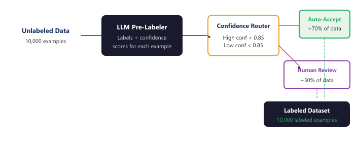
When using LLM pre-labels, always ask the model to output a confidence score alongside each label. Route examples with confidence below 0.7 directly to human review, and auto-accept examples above 0.95 with only spot-check audits. This "confidence-based triage" can reduce human annotation effort by 70% while maintaining label quality within 2% of full human annotation.
15.4.1.1 The Pre-Labeling Workflow
The pre-labeling workflow uses confidence-based routing to human review: high-confidence LLM labels are auto-accepted, mid-range labels are queued for human verification, and low-confidence labels are sent for full human labeling. The result is a noisy but rapidly-growing labeled dataset that can be cleaned with the noise-handling techniques covered later in this section.
Think of LLM-assisted labeling as hiring a teaching assistant to pre-grade exams. The TA (the LLM) makes a first pass over all submissions, marking answers with preliminary scores. The professor (the human annotator) then reviews and corrects the TA's work, focusing attention on borderline cases rather than obvious ones. Active learning is like the TA flagging the hardest questions and asking the professor to grade those first, maximizing the value of each minute of expert time. Code Fragment 15.4.2 shows this approach in practice.
The following implementation (Code Fragment 15.4.1a) shows this approach in practice.
Code Fragment 15.4.2b demonstrates the Batch API workflow.
# Structure annotation tasks as JSON with labeling guidelines
# Consistent formatting enables both human and LLM annotators
import json
from openai import OpenAI
from dataclasses import dataclass
client = OpenAI()
@dataclass
class PreLabel:
    text: str
    label: str
    confidence: float
    reasoning: str
def llm_prelabel(
    texts: list[str],
    label_options: list[str],
    task_description: str,
    model: str = "gpt-4o-mini"
    ) -> list[PreLabel]:
    """Pre-label a batch of texts using an LLM with confidence scores."""
    labels_str = ", ".join(f'"{l}"' for l in label_options)
results = []
for text in texts:
    prompt = f"""Task: {task_description}
    Text: "{text}"
    Available labels: [{labels_str}]
    Classify this text. Provide:
    1. The label (must be one of the available options)
    2. Your confidence (0.0 to 1.0)
    3. Brief reasoning
    Respond as JSON:
    {{
            "label": "chosen_label",
            "confidence": 0.95,
            "reasoning": "why this label"
            }}"""
    # Send chat completion request to the API
    response = client.chat.completions.create(
        model=model,
        messages=[{"role": "user", "content": prompt}],
        temperature=0.1,
        response_format={"type": "json_object"}
        )
    # Extract the generated message from the API response
    data = json.loads(response.choices[0].message.content)
    results.append(PreLabel(
            text=text,
            label=data["label"],
            confidence=data["confidence"],
            reasoning=data.get("reasoning", "")
            ))
    return results
# Example: Sentiment classification pre-labeling
texts = [
    "This product exceeded all my expectations. Highly recommend!",
    "The delivery was okay but the packaging was damaged.",
    "Worst purchase I have ever made. Complete waste of money.",
    "It does what it says. Nothing special, nothing terrible.",
    "I cannot figure out how to set this up. Instructions are unclear.",
    ]
prelabels = llm_prelabel(
    texts=texts,
    label_options=["positive", "negative", "neutral", "mixed"],
    task_description="Classify the sentiment of this product review."
    )
for pl in prelabels:
    route = "AUTO" if pl.confidence >= 0.85 else "HUMAN"
    print(f"[{route}] {pl.label} ({pl.confidence:.2f}): "
f"{pl.text[:50]}...")Code Fragment 15.4.2c establishes a ML baseline.
# Calculate annotation quality metrics using numpy
# Track agreement rates, label distributions, and annotator reliability
import numpy as np
from sklearn.metrics.pairwise import cosine_distances
def uncertainty_sampling(
    predictions: np.ndarray,
    n_select: int = 50
    ) -> np.ndarray:
    """Select examples where the model is most uncertain.
    Args:
    predictions: Array of shape (n_samples, n_classes) with
    predicted probabilities
    n_select: Number of examples to select
    Returns:
    Indices of selected examples
    """
    # Entropy-based uncertainty
    entropy = -np.sum(
        predictions * np.log(predictions + 1e-10), axis=1
    )
    # Select top-k most uncertain
    return np.argsort(entropy)[-n_select:]
def diversity_sampling(
    embeddings: np.ndarray,
    labeled_embeddings: np.ndarray,
    n_select: int = 50
    ) -> np.ndarray:
    """Select examples most different from the already-labeled set.
    Uses maximum distance to nearest labeled example (core-set approach).
    """
    # Distance from each unlabeled example to nearest labeled example
    distances = cosine_distances(embeddings, labeled_embeddings)
    min_distances = distances.min(axis=1)
    # Select the most distant (most different from labeled set)
    return np.argsort(min_distances)[-n_select:]
def hybrid_acquisition(
    predictions: np.ndarray,
    embeddings: np.ndarray,
    labeled_embeddings: np.ndarray,
    n_select: int = 50,
    uncertainty_weight: float = 0.6
    ) -> np.ndarray:
    """Hybrid strategy: weighted combination of uncertainty and diversity."""
    # Normalize uncertainty scores to [0, 1]
    entropy = -np.sum(predictions * np.log(predictions + 1e-10), axis=1)
    max_entropy = np.log(predictions.shape[1])
    uncertainty_scores = entropy / max_entropy
    # Normalize diversity scores to [0, 1]
    distances = cosine_distances(embeddings, labeled_embeddings)
    min_distances = distances.min(axis=1)
    diversity_scores = min_distances / max(min_distances.max(), 1e-10)
    # Weighted combination
    combined = (
        uncertainty_weight * uncertainty_scores +
        (1 - uncertainty_weight) * diversity_scores
    )
    return np.argsort(combined)[-n_select:]
# Simulate an active learning scenario
np.random.seed(42)
n_unlabeled = 1000
n_classes = 4
# Simulated model predictions (some confident, some uncertain)
predictions = np.random.dirichlet(np.ones(n_classes) * 2, n_unlabeled)
embeddings = np.random.randn(n_unlabeled, 128)
labeled_embeddings = np.random.randn(100, 128)
# Select using each strategy
uncertain_idx = uncertainty_sampling(predictions, n_select=50)
diverse_idx = diversity_sampling(embeddings, labeled_embeddings, n_select=50)
hybrid_idx = hybrid_acquisition(
    predictions, embeddings, labeled_embeddings, n_select=50
)
# Check overlap between strategies
overlap_u_d = len(set(uncertain_idx) & set(diverse_idx))
overlap_u_h = len(set(uncertain_idx) & set(hybrid_idx))
print(f"Uncertainty vs Diversity overlap: {overlap_u_d}/50 examples")
print(f"Uncertainty vs Hybrid overlap: {overlap_u_h}/50 examples")
print(f"Hybrid captures both uncertain AND diverse examples")The low overlap between uncertainty and diversity sampling (3 out of 50) demonstrates that these strategies target fundamentally different types of informative examples. Uncertainty sampling finds examples near decision boundaries, while diversity sampling finds examples in unexplored regions of the input space. The hybrid approach captures value from both, making it the recommended default for most practical applications.
15.4.1.2 The Acquisition Function and a Stopping Criterion
The code above selects examples by entropy, but to reproduce an active-learning loop you need the scoring rule stated precisely and a rule for when to stop. The problem is concrete: at every round you hold a pool of unlabeled examples and a fixed human-labeling budget, and you must decide which examples to send for annotation and when further annotation stops paying for itself. An acquisition function assigns each candidate a scalar informativeness score, and you label the top-k by that score.
The acquisition function used here is predictive entropy. Given the model's class-probability vector $p = (p_1, \dots, p_C)$ for an example, the entropy is
Entropy peaks when the distribution is uniform ($p_c = 1/C$ for all $c$, giving $H = \log C$) and falls to $0$ when one class has all the mass. Maximizing $H(p)$ therefore selects the examples on which the current model is most undecided, which are exactly the examples sitting near its decision boundaries. Two cheaper alternatives target the same intuition: least-confidence scores $1 - \max_c p_c$, and margin scores $-(p_{(1)} - p_{(2)})$ using the gap between the top two class probabilities. We use entropy because it accounts for the full distribution rather than just the top one or two classes, which matters when $C$ is larger than a handful. The Bayesian upgrade, BALD, scores the mutual information between an example's prediction and the model posterior, $I(y; \theta \mid x)$, isolating epistemic uncertainty (what the model does not know) from aleatoric noise (genuine label ambiguity that no amount of labeling will resolve).
The intuition is that a high-entropy example carries the most information per label because resolving it moves the decision boundary the most; labeling an example the model is already certain about teaches it almost nothing. Two failure modes follow directly. In the cold-start regime the model is untrained, so its probabilities are near-uniform everywhere and entropy ranks examples almost at random; seed the loop with a small random or diversity-sampled batch first. And pure uncertainty sampling is drawn to outliers and mislabeled noise, which are uncertain for the wrong reason, so pairing entropy with the diversity term from Code Fragment 15.4.2d guards against spending the budget on unrepresentative points.
A loop that never stops wastes budget, so we need a quantitative halting rule. A simple and robust stopping criterion watches the acquisition scores themselves: stop when the mean entropy of the selected top-k batch falls below a threshold $\tau$,
because once even the most uncertain remaining examples are confidently predicted, there is little left to learn. In practice $\tau$ is set as a fraction of the maximum possible entropy (for example $\tau = 0.25 \log C$). An alternative ties the stop to downstream value rather than to the pool: halt when the validation-accuracy gain per labeled batch drops below a tolerance $\epsilon$, since paying for labels that no longer move the metric is wasted effort.
Code Fragment 15.4.5 below makes the rule reproducible. Given a matrix of class probabilities it computes per-example entropy, selects the top-k by score, and reports both the chosen indices and the stopping check against $\tau$. It uses only NumPy so the arithmetic of the formula above is visible end to end.
# Entropy acquisition for active learning: score each example by
# predictive entropy, pick the top-k most uncertain, and apply a
# mean-entropy stopping rule. Pure NumPy so the formula is explicit.
import numpy as np

def predictive_entropy(probs: np.ndarray) -> np.ndarray:
    """H(p) = -sum_c p_c log p_c, computed per row (per example)."""
    # 1e-12 floor avoids log(0); abstaining rows would be handled upstream
    return -np.sum(probs * np.log(probs + 1e-12), axis=1)

def select_to_label(probs: np.ndarray, k: int):
    """Return the indices of the k highest-entropy examples and the
    mean entropy of that batch (the quantity the stop rule watches)."""
    scores = predictive_entropy(probs)
    # argsort ascending, take the last k -> the most uncertain
    topk = np.argsort(scores)[-k:][::-1]
    return topk, float(scores[topk].mean())

# Five examples over three classes, from confident to maximally uncertain
probs = np.array([
    [0.90, 0.05, 0.05],  # confident
    [0.34, 0.33, 0.33],  # near-uniform, high entropy
    [0.70, 0.20, 0.10],
    [0.45, 0.45, 0.10],  # two-way tie, high entropy
    [0.98, 0.01, 0.01],  # very confident
])

k = 2
selected, batch_mean_H = select_to_label(probs, k)
tau = 0.25 * np.log(probs.shape[1])  # 0.25 * log(C)

print(f"Per-example entropy: {np.round(predictive_entropy(probs), 3)}")
print(f"Selected to label (top-{k}): {selected.tolist()}")
print(f"Batch mean entropy: {batch_mean_H:.3f}  threshold tau: {tau:.3f}")
print(f"Stop? {batch_mean_H < tau}")predictive_entropy applies $H(p) = -\sum_c p_c \log p_c$ row-wise, select_to_label returns the top-k indices (here examples 1 and 3, the near-uniform and tied rows), and the batch mean entropy of 1.024 stays above the threshold $\tau = 0.25\log C \approx 0.275$, so the loop continues rather than stopping.15.4.2 Annotation Tools
Production annotation workflows require purpose-built tools that support team management, quality control, pre-labeling integration, and export in standard formats compatible with fine-tuning data preparation pipelines. The three leading tools for NLP annotation each serve different needs.
| Tool | License | Strengths | Best For | LLM Integration |
|---|---|---|---|---|
| Label Studio | Apache 2.0 | Highly customizable, multi-modal, large community | General purpose annotation across text, image, audio | ML backend API for pre-labeling |
| Prodigy | Commercial | Fast binary annotation, active learning built-in | Rapid iterative labeling with model-in-the-loop | Custom recipe system for LLM integration |
| Argilla | Apache 2.0 | Native LLM/NLP focus, HF Hub integration, Distilabel pairing | LLM output curation, preference labeling, RLHF data | First-class LLM pre-labeling support |
Code Fragment 15.4.3 demonstrates this approach.
# Label Studio: Setting up a pre-labeling backend with LLM
# This creates a backend service that Label Studio calls for predictions
from label_studio_ml.model import LabelStudioMLBase
from openai import OpenAI
class LLMPreLabeler(LabelStudioMLBase):
    """Label Studio ML backend that uses an LLM for pre-labeling."""
    def setup(self):
        self.client = OpenAI()
        self.model = "gpt-4o-mini"
    def predict(self, tasks, **kwargs):
        """Generate pre-labels for a batch of tasks."""
        predictions = []
        for task in tasks:
            text = task["data"].get("text", "")
            response = self.client.chat.completions.create(
                model=self.model,
                messages=[{
                "role": "user",
                "content": f"Classify the sentiment of this text as "
                f"'positive', 'negative', or 'neutral'.\n\n"
                f"Text: {text}\n\nLabel:"
                }],
                temperature=0.1,
                max_tokens=10
                )
            label = response.choices[0].message.content.strip().lower()
            predictions.append({
                "result": [{
                "from_name": "sentiment",
                "to_name": "text",
                "type": "choices",
                "value": {"choices": [label]}
                }],
                "score": 0.85 # Confidence score
                })
            return predictions
            # To run: label-studio-ml start ./llm_backend
            # Then connect in Label Studio: Settings > Machine Learning > Add Model
            print("LLM pre-labeling backend configured for Label Studio")
15.4.3 Inter-Annotator Agreement
When multiple annotators (human or LLM) label the same examples, measuring their agreement is essential for understanding label quality. Low agreement indicates ambiguous guidelines, difficult examples, or inconsistent annotators. High agreement (but not perfect) suggests well-calibrated labeling. Agreement metrics also help identify when LLM labels are reliable enough to substitute for human labels. Code Fragment 15.4.4 shows this approach in practice.
# Compute inter-annotator agreement using Cohen's kappa
# Kappa measures agreement beyond chance between two raters
import numpy as np
from itertools import combinations
def cohens_kappa(labels_a: list, labels_b: list) -> float:
    """Compute Cohen's Kappa between two annotators."""
    assert len(labels_a) == len(labels_b)
    n = len(labels_a)
    # Observed agreement
    observed = sum(a == b for a, b in zip(labels_a, labels_b)) / n
    # Expected agreement (by chance)
    unique_labels = set(labels_a) | set(labels_b)
    expected = 0
    for label in unique_labels:
        freq_a = labels_a.count(label) / n
        freq_b = labels_b.count(label) / n
        expected += freq_a * freq_b
        if expected == 1.0:
            return 1.0
            return (observed - expected) / (1 - expected)
def fleiss_kappa(ratings_matrix: np.ndarray) -> float:
    """Compute Fleiss' Kappa for multiple annotators.
    Args:
    ratings_matrix: Shape (n_subjects, n_categories).
    Each cell is the count of raters who assigned
    that category to that subject.
    """
    n_subjects, n_categories = ratings_matrix.shape
    n_raters = ratings_matrix.sum(axis=1)[0] # Assume same per subject
    # Proportion of assignments to each category
    p_j = ratings_matrix.sum(axis=0) / (n_subjects * n_raters)
    # Per-subject agreement
    p_i = (
        (ratings_matrix ** 2).sum(axis=1) - n_raters
        ) / (n_raters * (n_raters - 1))
    p_bar = p_i.mean()
    p_e = (p_j ** 2).sum()
    if p_e == 1.0:
        return 1.0
        return (p_bar - p_e) / (1 - p_e)
        # Example: Compare LLM labels with two human annotators
        human_a = ["pos", "neg", "neu", "pos", "neg", "pos", "neu", "neg", "pos", "neu"]
        human_b = ["pos", "neg", "pos", "pos", "neg", "pos", "neg", "neg", "pos", "neu"]
        llm = ["pos", "neg", "neu", "pos", "neg", "pos", "neu", "neg", "pos", "pos"]
        kappa_humans = cohens_kappa(human_a, human_b)
        kappa_llm_a = cohens_kappa(llm, human_a)
        kappa_llm_b = cohens_kappa(llm, human_b)
        print(f"Human A vs Human B (Kappa): {kappa_humans:.3f}")
        print(f"LLM vs Human A (Kappa): {kappa_llm_a:.3f}")
        print(f"LLM vs Human B (Kappa): {kappa_llm_b:.3f}")
        print()
        print("Interpretation:")
        print(" 0.81-1.00: Almost perfect agreement")
        print(" 0.61-0.80: Substantial agreement")
        print(" 0.41-0.60: Moderate agreement")
        print(" 0.21-0.40: Fair agreement")
print(" < 0.20: Slight/poor agreement")High LLM-human agreement does not always mean high quality. If the LLM and a single annotator agree strongly but disagree with other annotators, the LLM may be mimicking that annotator's biases rather than capturing ground truth. Always measure agreement against multiple independent annotators and investigate cases where LLM labels differ from the human majority vote.
Active learning selects the most informative examples for human review, which means your annotators spend their time on the hard cases instead of labeling obvious ones. It is like a teacher who only grades the essays they suspect might be plagiarized.
LLM pre-labeling changes the economics of annotation without replacing human judgment. The key insight is that LLMs are surprisingly good at easy cases (where annotators would agree anyway) but unreliable on genuinely ambiguous examples. Active learning exploits this asymmetry: let the LLM handle the 70% of straightforward cases, and route the uncertain 30% to human annotators. This approach typically delivers 3x to 5x annotation speedup while maintaining or improving label quality, because human attention is concentrated on the examples that actually need expert judgment.
Who: A product analytics team at a consumer electronics company analyzing 500,000 product reviews per quarter across 12 product lines.
Situation: They needed fine-grained sentiment labels (positive, negative, neutral, mixed) plus aspect tags (battery, screen, camera, price, durability) for each review. Manual annotation by a team of 8 contractors achieved 90% accuracy but could only process 2,000 reviews per week.
Problem: At the current annotation rate, labeling one quarter's reviews would take over 4 years. They needed a 50x speedup without significant quality loss.
Dilemma: They could use an LLM for all labeling (fast but 82% accuracy on their domain-specific aspect tags), train annotators to review LLM suggestions rather than label from scratch (faster but still limited by headcount), or combine LLM pre-labeling with active learning to minimize human effort.
Decision: They implemented a three-phase pipeline: (1) GPT-4o-mini pre-labeled all 500,000 reviews with confidence scores, (2) active learning selected the 15,000 most informative examples for human review using uncertainty sampling plus diversity sampling, and (3) a fine-tuned DeBERTa model trained on the corrected labels processed the full corpus.
How: The LLM pre-labeled the full batch in 6 hours using the batch API at 50% discount. Annotators reviewed LLM suggestions (correcting rather than creating labels), achieving 5x their normal throughput (10,000 reviews per week). Active learning prioritized reviews where the LLM was uncertain (confidence below 0.7) and reviews from underrepresented product categories.
Result: The fine-tuned DeBERTa model achieved 88% accuracy on aspect-level sentiment (compared to 82% for GPT-4o-mini alone and 90% for full human annotation). Total annotation cost was $18,000 instead of the estimated $450,000 for full manual labeling, a 96% reduction. The full pipeline from raw reviews to labeled dataset took 3 weeks.
Lesson: Active learning multiplies the value of every human annotation by focusing reviewer time on the examples where corrections have the greatest impact on model quality; LLM pre-labeling changes the annotator's task from creation to verification, which is fundamentally faster.
Active learning with LLM labelers is converging with curriculum learning strategies, where the difficulty and diversity of selected examples are jointly optimized for maximum training efficiency.
Recent work on calibrated LLM confidence enables more principled uncertainty sampling by producing reliable probability estimates for when labels need human review. The frontier challenge is developing active learning loops that can simultaneously select informative examples and detect systematic labeling errors from the LLM annotator.
- LLM pre-labeling speeds up annotation 2x to 5x by providing initial labels that human reviewers correct rather than create from scratch.
- Confidence-based routing auto-accepts high-confidence labels and sends uncertain examples to humans. The threshold must be calibrated on held-out gold data, not based on the model's self-reported confidence.
- Active learning reduces annotation costs by 40% to 70% by selecting the most informative examples. The hybrid strategy (uncertainty + diversity) captures value from both decision boundary refinement and input space exploration.
- Three leading annotation tools serve different needs: Label Studio (general purpose, multi-modal), Prodigy (fast iterative labeling), and Argilla (LLM-native, RLHF data).
- Inter-annotator agreement (Cohen's Kappa, Fleiss' Kappa) measures label quality. Always compare LLM labels against multiple independent human annotators, not just one.
Show Answer
Show Answer
Show Answer
Show Answer
Show Answer
Exercises
Explain the difference between using an LLM to directly label data versus using an LLM to pre-label data for human review. When is each approach appropriate?
Answer Sketch
Direct LLM labeling: the LLM's labels are used as ground truth without human review. Appropriate for low-stakes tasks where 85 to 90% accuracy is acceptable (e.g., content tagging for internal analytics). Pre-labeling: the LLM generates initial labels that humans verify and correct. Appropriate for high-stakes tasks (medical, legal) where accuracy must exceed 95%. Pre-labeling speeds up human annotation by 3 to 5x because reviewers correct rather than create labels from scratch.
Describe how active learning can be combined with LLM labeling. How do you select which examples the LLM should label versus which need human review?
Answer Sketch
Train an initial classifier on a small labeled set. For each unlabeled example, compute the classifier's uncertainty (e.g., entropy of class probabilities). High-uncertainty examples go to human annotators (the model needs help on these). Low-uncertainty examples are labeled by the LLM (the task is straightforward). Medium-uncertainty examples are labeled by the LLM with human spot-checks. This focuses expensive human effort on the examples that provide the most training signal.
Write a function that measures inter-annotator agreement between an LLM labeler and human labels using Cohen's kappa. Include interpretation of the kappa score.
Answer Sketch
Use from sklearn.metrics import cohen_kappa_score. Compute kappa = cohen_kappa_score(human_labels, llm_labels). Interpret: kappa < 0.2 = slight agreement, 0.2 to 0.4 = fair, 0.4 to 0.6 = moderate, 0.6 to 0.8 = substantial, > 0.8 = almost perfect. If kappa < 0.6, the LLM labels are too unreliable for direct use and need human review. Also compute per-class F1 to identify which categories the LLM struggles with.
You have a budget of $5,000 to label 100,000 examples. Human labeling costs $0.10/example (50,000 affordable). LLM labeling costs $0.005/example (all 100K affordable). Design a labeling strategy that maximizes quality within budget.
Answer Sketch
Label 10,000 examples with humans ($1,000) as a gold standard. Use the LLM to label all 100,000 ($500). Compare LLM labels to human labels on the 10K overlap; identify error patterns. Spend the remaining $3,500 on human review of the LLM's least confident predictions (35,000 reviews). Final dataset: 35,000 human-verified + 65,000 LLM-labeled (with known accuracy from the calibration set). Total cost: $5,000.
Write Python code that assesses whether an LLM labeler's confidence scores are well-calibrated. Plot a reliability diagram (predicted confidence vs. actual accuracy) using 10 bins.
Answer Sketch
Bin LLM predictions by stated confidence (0.0 to 0.1, 0.1 to 0.2, etc.). For each bin, compute the fraction of predictions that are actually correct (vs. human ground truth). Plot bin midpoints (x) vs. actual accuracy (y). A perfectly calibrated model lies on the diagonal. Use matplotlib to plot with a reference diagonal line. Compute Expected Calibration Error (ECE) as the weighted average of |accuracy - confidence| per bin.
What Comes Next
In the next section, Section 15.5: Weak Supervision & Programmatic Labeling, we explore weak supervision and programmatic labeling, scaling annotation through heuristic rules and model-generated labels. The active learning loop described here also benefits from the human-in-the-loop feedback patterns in Section 18.1.