Section 19.3 cataloged the datasets and benchmarks Part IV draws on, plus the lightweight DVC versioning workflow. This section covers the heavyweight tooling you need once those datasets stop fitting on one machine: PySpark for distributed text preprocessing, Delta Lake for ACID storage on S3, and feature stores for training-serving consistency. The three layers stack: Spark reads from and writes to Delta tables; feature stores materialize features from Delta into low-latency online stores. Pick one tool from each layer.
PySpark for LLM Data Pipelines
Training and fine-tuning LLMs requires processing corpora that range from tens of gigabytes to multiple terabytes. PySpark provides the distributed compute layer that makes this tractable: it parallelizes text cleaning, deduplication, tokenization, and embedding generation across hundreds of cores, and it integrates naturally with the Delta Lake storage layer covered later in this section and the Databricks platform from Section 19.1. This section walks through each stage of a PySpark-based LLM data pipeline, from reading raw corpora to writing training-ready Parquet files and populating vector databases.
O.1.1 PySpark Fundamentals for Text Data
Before processing any text, configure your SparkSession for the memory profiles that
LLM data pipelines demand. Text data is wide (long strings), so default Spark settings for shuffle
partitions and executor memory are often too conservative.
from pyspark.sql import SparkSession
from pyspark.sql import functions as F
from pyspark.sql.types import StringType, FloatType, IntegerType

# Configure SparkSession for LLM data workloads
spark = (
    SparkSession.builder
    .appName("llm-data-pipeline")
    # Increase shuffle partitions for large text corpora
    .config("spark.sql.shuffle.partitions", "800")
    # Allow Spark to read ORC/Parquet metadata without loading full columns
    .config("spark.sql.parquet.filterPushdown", "true")
    # Use Kryo for faster serialization of Python objects
    .config("spark.serializer", "org.apache.spark.serializer.KryoSerializer")
    # Driver and executor memory: tune to your cluster
    .config("spark.driver.memory", "16g")
    .config("spark.executor.memory", "32g")
    .config("spark.executor.memoryOverhead", "4g")
    # Adaptive Query Execution (Spark 3+): auto-coalesces small partitions
    .config("spark.sql.adaptive.enabled", "true")
    .config("spark.sql.adaptive.coalescePartitions.enabled", "true")
    .getOrCreate()
)

spark.sparkContext.setLogLevel("WARN")# Read from Delta Lake (recommended for managed pipelines)
df_delta = spark.read.format("delta").load("s3://my-bucket/corpora/c4-en")
# Read from Parquet (e.g., downloaded Common Crawl snapshots)
df_parquet = spark.read.parquet("s3://my-bucket/raw/cc-2024-10/")
# Read from newline-delimited JSON
df_json = (
spark.read
.option("multiline", "false") # one JSON object per line
.json("s3://my-bucket/raw/dolma-v1.7/")
)
# Read from CSV with header (e.g., OpenWebText metadata)
df_csv = (
spark.read
.option("header", "true")
.option("inferSchema", "true")
.csv("s3://my-bucket/raw/openwebtext-meta/")
)
# Quick schema inspection
df_delta.printSchema()
print(f"Row count: {df_delta.count():,}")import torch.nn.functional as F
# Filter to English, require minimum text length and quality score
df_filtered = (
df_delta
.filter(F.col("language") == "en")
.filter(F.col("language_score") >= 0.85)
.filter(F.length("text") >= 200)
.filter(F.length("text") <= 100_000)
.filter(F.col("quality_score") >= 0.5)
)
# Register a UDF for language detection on raw text (when no pre-computed label)
from langdetect import detect, LangDetectException
def detect_lang(text: str) -> str:
if not text or len(text) < 20:
return "unknown"
try:
return detect(text)
except LangDetectException:
return "unknown"
detect_lang_udf = F.udf(detect_lang, StringType())
df_with_lang = df_json.withColumn("detected_lang", detect_lang_udf(F.col("text")))
df_en = df_with_lang.filter(F.col("detected_lang") == "en")
PySpark can read all common corpus formats. Delta Lake is preferred for its ACID guarantees and time-travel capabilities (see this section), but raw Parquet and JSON are also common for externally sourced datasets.
Basic DataFrame operations for text quality gating run as distributed SQL-style transformations.
Language filtering, length thresholding, and quality score cuts are all expressible with
F.col predicates and are pushed down to the storage layer when reading Parquet.
import torch.nn.functional as F
import hashlib
from pyspark.ml.feature import MinHashLSH, HashingTF, Tokenizer
from pyspark.sql.functions import col, udf
from pyspark.sql.types import StringType
# --- Exact deduplication via SHA-256 ---
def sha256_hash(text: str) -> str:
    return hashlib.sha256(text.encode("utf-8")).hexdigest()
hash_udf = F.udf(sha256_hash, StringType())
df_hashed = df_filtered.withColumn("doc_hash", hash_udf(F.col("text")))
# Keep only the first occurrence of each hash
from pyspark.sql.window import Window
window = Window.partitionBy("doc_hash").orderBy("url")
df_exact_deduped = (
    df_hashed
    .withColumn("rank", F.row_number().over(window))
    .filter(F.col("rank") == 1)
    .drop("rank")
    )
print(f"After exact dedup: {df_exact_deduped.count():,} docs")
After exact deduplication trims the corpus to the documents that have unique SHA-256 hashes, the second stage targets near-duplicates that survived the exact pass (paraphrases, light edits, formatting differences) via MinHash LSH.
import torch.nn.functional as F
# --- Near-duplicate removal via MinHash LSH ---
# Tokenize into word shingles
tokenizer = Tokenizer(inputCol="text", outputCol="words")
df_words = tokenizer.transform(df_exact_deduped)
# Hash shingles into a feature vector
hashing_tf = HashingTF(inputCol="words", outputCol="features", numFeatures=262144)
df_features = hashing_tf.transform(df_words)
# Build MinHash LSH model
mh = MinHashLSH(inputCol="features", outputCol="hashes", numHashTables=5)
model = mh.fit(df_features)
# Find near-duplicate pairs (Jaccard similarity >= 0.8)
df_pairs = model.approxSimilarityJoin(
df_features, df_features,
threshold=0.2, # distance threshold = 1 - 0.8 Jaccard
distCol="distance"
)
# Extract IDs of duplicates to remove (keep lowest ID in each cluster)
duplicates_to_remove = (
df_pairs
.filter(F.col("datasetA.id") != F.col("datasetB.id"))
.select(F.greatest("datasetA.id", "datasetB.id").alias("remove_id"))
.distinct()
)
df_near_deduped = df_features.join(
duplicates_to_remove,
df_features["id"] == duplicates_to_remove["remove_id"],
how="left_anti"
)Row-level Python UDFs incur Python-JVM serialization overhead for every row. For high-throughput pipelines, prefer pandas_udf (covered in O.1.3 and O.1.4) which processes batches of rows using Arrow, reducing overhead by 10-50x.
O.1.2 Large-Scale Text Preprocessing
Raw web corpora contain near-duplicate documents, malformed HTML, non-standard Unicode, and personally identifiable information (PII). Removing these before tokenization is essential for training data quality and legal compliance.
Deduplication
Exact deduplication uses a hash of the document content. Near-duplicate removal requires MinHash Locality Sensitive Hashing (LSH), which approximates Jaccard similarity between documents at scale.
import torch.nn.functional as F
import pandas as pd
from pyspark.sql.types import StructType, StructField
SEQ_LEN = 4096
EOS_ID = 2 # Llama EOS token ID
@pandas_udf(ArrayType(IntegerType()))
def pack_sequences(token_id_lists: pd.Series) -> pd.Series:
    """Greedily pack variable-length token sequences into fixed-length chunks."""
    packed = []
    current_chunk = []
    for token_ids in token_id_lists:
        if not token_ids:
            continue
        # Append EOS after each document
        doc_tokens = list(token_ids) + [EOS_ID]
        # Split document if longer than context window
        while len(doc_tokens) > 0:
            space = SEQ_LEN - len(current_chunk)
            current_chunk.extend(doc_tokens[:space])
            doc_tokens = doc_tokens[space:]
            if len(current_chunk) == SEQ_LEN:
                packed.append(current_chunk)
                current_chunk = []
                # Discard the final partial chunk (do not pad)
                return pd.Series(packed)
            df_packed = df_tokenized.groupBy("partition_id").agg(
                pack_sequences(F.col("token_ids")).alias("packed_sequences")
                )
pack_sequences UDF concatenates variable-length documents with EOS separators into fixed-length windows of SEQ_LEN tokens, improving GPU utilization by 15 to 30% compared to per-document truncation with padding.Text Cleaning and PII Redaction
import torch.nn.functional as F
import re
import unicodedata
from pyspark.sql.functions import pandas_udf
import pandas as pd
# Regex patterns for PII and noise
EMAIL_RE = re.compile(r"[a-zA-Z0-9_.+-]+@[a-zA-Z0-9-]+\.[a-zA-Z0-9-.]+")
PHONE_RE = re.compile(r"\b(\+?1[\s.-]?)?\(?\d{3}\)?[\s.-]?\d{3}[\s.-]?\d{4}\b")
HTML_TAG_RE = re.compile(r"<[^>]+>")
MULTI_SPACE_RE = re.compile(r"\s+")
@pandas_udf(StringType())
def clean_text(texts: pd.Series) -> pd.Series:
    def _clean(text: str) -> str:
        if not isinstance(text, str):
            return ""
        # Strip HTML tags
        text = HTML_TAG_RE.sub(" ", text)
        # Normalize Unicode to NFC form
        text = unicodedata.normalize("NFC", text)
        # Redact PII
        text = EMAIL_RE.sub("[EMAIL]", text)
        text = PHONE_RE.sub("[PHONE]", text)
        # Collapse whitespace
        text = MULTI_SPACE_RE.sub(" ", text).strip()
        return text
    return texts.apply(_clean)
df_cleaned = df_near_deduped.withColumn("text", clean_text(F.col("text")))
pandas_udf. Processing a Pandas Series per partition is significantly faster than row-level UDFs for regex-heavy operations.import torch.nn.functional as F
from transformers import AutoTokenizer
from pyspark.sql.types import ArrayType, IntegerType
import pandas as pd
MODEL_NAME = "meta-llama/Llama-3.1-8B"
TOKENIZER_BROADCAST = None # populated per-partition to avoid serialization
@pandas_udf(ArrayType(IntegerType()))
def tokenize_text(texts: pd.Series) -> pd.Series:
# Load tokenizer once per executor process (cached after first call)
global TOKENIZER_BROADCAST
if TOKENIZER_BROADCAST is None:
TOKENIZER_BROADCAST = AutoTokenizer.from_pretrained(
MODEL_NAME, use_fast=True
)
tok = TOKENIZER_BROADCAST
# Tokenize the whole batch at once (fast tokenizers support batching)
results = tok(
texts.tolist(),
truncation=False,
padding=False,
add_special_tokens=False,
)
return pd.Series(results["input_ids"])
df_tokenized = df_cleaned.withColumn("token_ids", tokenize_text(F.col("text")))
pandas_udf. The tokenizer is loaded once per executor process using a global variable. Using use_fast=True enables the Rust-backed tokenizer, which is 5 to 10x faster than the Python implementation.The C4 dataset (used to train T5 and many subsequent models) applies a sequence of quality filters that are straightforward to replicate in PySpark:
- Keep only lines ending in terminal punctuation (
.,!,?,"). - Remove documents with fewer than 5 sentences or fewer than 3 words per line on average.
- Remove documents containing any of a list of profanity/toxic keywords.
- Remove lines containing the substring
javascript(catches boilerplate web page noise).
Each filter is a simple F.col predicate or a single-pass UDF and adds negligible compute cost relative to the I/O required to read the corpus.
O.1.3 Tokenization and Dataset Preparation
Once text is cleaned and deduplicated, the next step is converting it into token sequences that
training frameworks can consume. Hugging Face tokenizers are the de facto standard; applying them
at scale requires wrapping them in a pandas_udf so the tokenizer is loaded once per
Spark partition rather than once per row.
# Write packed sequences to Parquet with tuned row group sizes
OUTPUT_PATH = "s3://my-bucket/training/llama-sft-packed-v3"

(
    df_packed
    .write
    .mode("overwrite")
    .option("parquet.block.size", 128 * 1024 * 1024)   # 128 MB row groups
    .option("parquet.page.size",  1 * 1024 * 1024)     # 1 MB pages
    .parquet(OUTPUT_PATH)
)

# --- In your training script, load directly as a HuggingFace Dataset ---
from datasets import load_dataset

dataset = load_dataset(
    "parquet",
    data_files={"train": f"{OUTPUT_PATH}/*.parquet"},
    split="train",
    num_proc=8,
)
print(dataset)
# Dataset({features: ['packed_sequences'], num_rows: 4200000})Dataset via the parquet loader. The 128 MB row group setting balances metadata overhead against read parallelism.Training efficiency requires packing multiple short documents into fixed-length sequences to avoid wasting context window capacity on padding tokens. The following UDF implements a greedy bin-packing approach per partition.
import torch
import numpy as np
import pandas as pd
from pyspark.sql.types import ArrayType, FloatType
from pyspark.sql.functions import pandas_udf, col
from sentence_transformers import SentenceTransformer

EMBEDDING_MODEL = "BAAI/bge-large-en-v1.5"
EMBED_DIM = 1024
BATCH_SIZE = 256   # tune to GPU memory

# Module-level cache: populated once per executor JVM process
_model_cache: dict = {}

@pandas_udf(ArrayType(FloatType()))
def embed_texts(texts: pd.Series) -> pd.Series:
    global _model_cache
    if EMBEDDING_MODEL not in _model_cache:
        device = "cuda" if torch.cuda.is_available() else "cpu"
        _model_cache[EMBEDDING_MODEL] = SentenceTransformer(
            EMBEDDING_MODEL, device=device
        )
    model = _model_cache[EMBEDDING_MODEL]

    # Process in mini-batches to avoid OOM on large partitions
    all_embeddings = []
    text_list = texts.tolist()
    for i in range(0, len(text_list), BATCH_SIZE):
        batch = text_list[i : i + BATCH_SIZE]
        embs = model.encode(
            batch,
            batch_size=len(batch),
            normalize_embeddings=True,
            show_progress_bar=False,
        )
        all_embeddings.extend(embs.tolist())

    return pd.Series(all_embeddings)

# Repartition to align one partition per GPU worker
df_embedded = (
    df_cleaned
    .select("id", "text", "url")
    .repartition(spark.sparkContext.defaultParallelism)
    .withColumn("embedding", embed_texts(col("text")))
)_model_cache dict ensures the model is loaded once per executor process, regardless of how many tasks that executor runs. Repartitioning to match GPU count minimizes model-load overhead.Converting to Hugging Face Datasets
The most efficient conversion path from Spark to a Hugging Face Dataset uses Apache
Arrow, which both Spark and Hugging Face natively support. Write Parquet from Spark, then load
with datasets.load_dataset.
Row group size directly affects streaming throughput. Groups that are too small increase metadata overhead; groups that are too large reduce parallelism when reading. The 128 MB default is a good starting point for single-GPU training. See this section for Delta Lake-specific Parquet optimization settings.
O.1.4 Embedding Generation at Scale
Generating embeddings for millions of documents is one of the most GPU-intensive offline tasks in
LLM infrastructure. The key challenge is loading the embedding model exactly once per Spark
executor (not once per row or even once per batch), and using Arrow-based pandas_udf
to send large batches to the GPU efficiently. This pattern connects directly to the vector search
infrastructure covered in Chapter 31.
Writing Embeddings and Ingesting into Vector Databases
# Write embeddings to Parquet for offline use
EMBED_PATH = "s3://my-bucket/embeddings/bge-large-v1"

(
    df_embedded
    .write
    .mode("overwrite")
    .parquet(EMBED_PATH)
)

# --- Batch upsert to Pinecone ---
import pinecone
from pyspark.sql.functions import struct

PINECONE_API_KEY = "..."
INDEX_NAME = "docs-bge-large"

def upsert_to_pinecone(rows):
    """Called once per Spark partition to batch-upsert embeddings."""
    pc = pinecone.Pinecone(api_key=PINECONE_API_KEY)
    index = pc.Index(INDEX_NAME)

    batch = []
    for row in rows:
        batch.append({
            "id": row["id"],
            "values": row["embedding"],
            "metadata": {"url": row["url"]},
        })
        if len(batch) == 200:
            index.upsert(vectors=batch)
            batch = []
    if batch:
        index.upsert(vectors=batch)

# foreachPartition loads the Pinecone client once per partition
df_embedded.foreachPartition(upsert_to_pinecone)foreachPartition. The same partition-level pattern works for Weaviate (using weaviate.batch) and Milvus (using pymilvus.Collection.insert).Use foreachPartition rather than foreach when writing to external systems like vector databases. foreach calls your function once per row, which causes one network round-trip per document. foreachPartition calls your function once per partition with an iterator, enabling batched writes and connection reuse that reduce total ingestion time by orders of magnitude.
O.1.5 Monitoring and Optimizing Spark Jobs
Even well-designed PySpark pipelines require tuning when run on real corpora. The Spark UI is the primary diagnostic tool; understanding its output is essential for identifying and fixing the bottlenecks most common in LLM data pipelines.
Using the Spark UI
The Spark UI is available at http://<driver-host>:4040 during a running job. On
Databricks, it is accessible via the cluster detail page. The most useful views for LLM pipeline
debugging are:
- Stages tab: shows per-stage task duration distributions. A long tail in the distribution indicates partition skew (one partition is much larger than others).
- SQL tab: shows the physical query plan with operator-level timing. Look for
BroadcastNestedLoopJoinas a warning sign that a join predicate was missed. - Executors tab: shows GC time per executor. GC time above 10% of task time usually indicates that executor heap size needs to increase or that large objects are being created per row.
- Storage tab: shows cached RDD/DataFrame sizes. If a DataFrame you intend to
reuse is not cached, adding
.cache()before the second use avoids recomputing it.
Common Bottlenecks in LLM Data Pipelines
# --- Diagnosing and fixing partition skew ---
# Check partition sizes after a wide transformation
from pyspark.sql.functions import spark_partition_id

partition_sizes = (
    df_cleaned
    .withColumn("pid", spark_partition_id())
    .groupBy("pid")
    .count()
    .orderBy("count", ascending=False)
)
partition_sizes.show(20)

# If max partition >> median, salt the skewed key
# Example: language="en" dominates. Salt with a random integer.
import pyspark.sql.functions as F

SALT_BUCKETS = 50
df_salted = df_cleaned.withColumn(
    "lang_salted",
    F.concat(F.col("language"), F.lit("_"), (F.rand() * SALT_BUCKETS).cast("int"))
)

# --- Broadcast join for small lookup tables ---
# Use when one side of a join is small (e.g., a domain blocklist)
from pyspark.sql.functions import broadcast

df_blocklist = spark.read.parquet("s3://my-bucket/blocklist/")  # small table

df_clean_domains = df_cleaned.join(
    broadcast(df_blocklist),
    on="domain",
    how="left_anti"  # exclude rows matching the blocklist
)

# --- Tune partition count for large shuffles ---
# Rule of thumb: target 100-200 MB per partition after shuffle
# For a 2 TB corpus with 200 MB target:
spark.conf.set("spark.sql.shuffle.partitions", str(2000 * 1024 // 200))Python UDFs serialize each row as a Python object, cross the JVM-Python boundary, execute the Python function, and serialize the result back. On a 1 TB corpus this overhead can be the dominant cost in your pipeline. Always profile with the Spark UI before adding UDFs, and prefer built-in Spark SQL functions (F.regexp_replace, F.length, etc.) when they cover your use case. Reserve Python UDFs for logic that genuinely cannot be expressed with built-ins, and use pandas_udf for everything else.
Cost Optimization
# --- Databricks cluster autoscaling configuration (JSON, not Python) ---
# Set in cluster creation API or Databricks UI
CLUSTER_CONFIG = {
    "cluster_name": "llm-data-pipeline",
    "spark_version": "15.4.x-scala2.12",
    "node_type_id": "i3.2xlarge",
    "autoscale": {
        "min_workers": 4,
        "max_workers": 40,
    },
    "aws_attributes": {
        "availability": "SPOT_WITH_FALLBACK",
        "spot_bid_price_percent": 100,
        "first_on_demand": 2,   # keep 2 on-demand nodes as stable driver/coordinator
    },
    "spark_conf": {
        "spark.sql.adaptive.enabled": "true",
        "spark.sql.adaptive.coalescePartitions.enabled": "true",
    },
}

# --- Checkpoint long pipelines to avoid recomputation on failure ---
spark.sparkContext.setCheckpointDir("s3://my-bucket/checkpoints/")

# Checkpoint after the expensive deduplication stage
df_near_deduped.checkpoint()   # materializes to S3, breaks lineage graph

# --- Cache DataFrames used more than once ---
df_tokenized.cache()
df_tokenized.count() # trigger materialization immediatelyFor pipelines that process a corpus incrementally (new data arriving daily), use Delta Lake's MERGE INTO operation rather than reprocessing the entire corpus each run. Combined with Delta's change data feed, you can identify only new or updated documents and pass them through the expensive deduplication and tokenization stages. This is covered in detail in this section.
Summary
PySpark provides the distributed compute foundation for every stage of an LLM data pipeline.
The SparkSession configuration choices in O.1.1 set the foundation for throughput and
memory stability. Deduplication via exact hashing and MinHash LSH in O.1.2 is the most impactful
single quality intervention for pretraining data. The pandas_udf pattern for
tokenization and embedding generation in O.1.3 and O.1.4 bridges PySpark with the Hugging Face
and SentenceTransformer ecosystems without sacrificing throughput. Finally, the Spark UI
diagnostics and tuning patterns in O.1.5 give you the tools to identify and eliminate the
bottlenecks that emerge when pipelines move from prototype to production scale.
These techniques integrate directly with the Databricks platform (this section), Delta Lake storage and ACID semantics (this section), and the Hugging Face Datasets library for downstream training (Hugging Face Transformers). For the vector search applications that consume the embeddings produced here, see Chapter 31.
Delta Lake and Lakehouse Architecture
Delta Lake is an open-source storage layer that brings ACID transactions, schema enforcement, and time travel to data lakes built on Parquet files. The Lakehouse architecture combines the low-cost scalability of data lakes with the reliability and performance features of data warehouses, creating a single platform for both analytics and ML. For LLM teams, Delta Lake provides versioned, auditable training datasets, efficient streaming ingestion of user feedback, and the foundation for reproducible training pipelines.
O.2.1 Why Data Lakes Alone Are Not Enough
Traditional data lakes store files (CSV, JSON, Parquet) in object storage like S3 or ADLS. While cheap and scalable, they lack the guarantees that ML pipelines demand. Without transactions, a concurrent write can corrupt a dataset mid-training. Without schema enforcement, an upstream change can silently add a column that breaks your tokenizer. Without versioning, you cannot answer the question "what exact data did we use to train model v2.3?"
Delta Lake solves these problems by adding a transaction log (the _delta_log directory)
on top of Parquet files. Every write operation, whether an insert, update, delete, or schema change,
is recorded as a JSON commit in this log. Readers consult the log to determine which Parquet files
constitute the current version of the table, providing snapshot isolation without a database server.
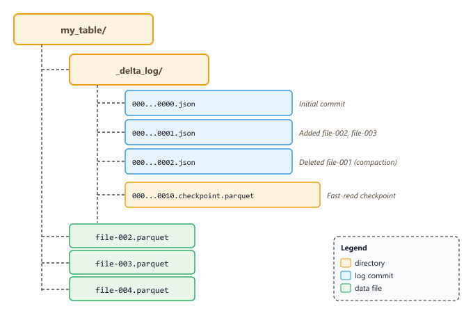
_delta_log directory contains ordered JSON commits that track every mutation. Checkpoint files accelerate log replay for tables with many commits.O.2.2 ACID Transactions and Concurrent Writes
Delta Lake uses optimistic concurrency control. When two writers attempt to modify the same table simultaneously, the first to commit wins, and the second must retry against the updated state. This guarantees that readers always see a consistent snapshot, even during active writes. For ML teams, this means a data engineer can append new training examples while a training job reads the table, without either operation blocking or corrupting the other.
from delta import DeltaTable
from pyspark.sql import SparkSession

spark = (SparkSession.builder
    .config("spark.jars.packages", "io.delta:delta-spark_2.12:3.1.0")
    .config("spark.sql.extensions", "io.delta.sql.DeltaSparkSessionExtension")
    .config("spark.sql.catalog.spark_catalog",
            "org.apache.spark.sql.delta.catalog.DeltaCatalog")
    .getOrCreate())

# Write a DataFrame as a Delta table
training_data = spark.read.json("s3://bucket/raw/instruction_pairs/")
training_data.write.format("delta").mode("overwrite").save(
    "s3://bucket/delta/instruction_pairs"
)

# Append new data (transactional, safe with concurrent readers)
new_examples = spark.read.json("s3://bucket/raw/new_batch_2024_03/")
new_examples.write.format("delta").mode("append").save(
    "s3://bucket/delta/instruction_pairs"
)Delta Lake's ACID transactions solve the "training data corruption" problem that plagues raw data lakes. Without transactions, a crash during a multi-file write can leave the dataset in an inconsistent state, which produces silent data quality issues that surface only as degraded model performance weeks later.
O.2.3 Time Travel for Reproducible Training
Every commit in the Delta log creates a new version of the table. You can query any historical version by specifying a version number or a timestamp. This feature, called time travel, is indispensable for ML reproducibility. When you log the Delta table version alongside your MLflow run (see this section), you can reconstruct the exact training dataset months or years later.
# Read a specific version of the Delta table
df_v5 = (spark.read.format("delta")
    .option("versionAsOf", 5)
    .load("s3://bucket/delta/instruction_pairs"))

# Read the table as it existed at a specific timestamp
df_historical = (spark.read.format("delta")
    .option("timestampAsOf", "2025-01-15T00:00:00Z")
    .load("s3://bucket/delta/instruction_pairs"))

# View the full commit history
delta_table = DeltaTable.forPath(spark, "s3://bucket/delta/instruction_pairs")
history = delta_table.history()
history.select("version", "timestamp", "operation", "operationMetrics").show(10)

# Restore the table to a previous version (useful for rollbacks)
delta_table.restoreToVersion(5)In your training scripts, always log the Delta table version alongside your model artifacts. A simple mlflow.log_param("delta_version", delta_table.history(1).first()["version"]) creates a permanent link between the model and its training data, enabling full reproducibility.
O.2.4 Schema Evolution and Enforcement
Delta Lake enforces schemas by default: if you attempt to write data with columns that do not match the table schema, the write fails with a clear error. This prevents the subtle bugs that occur when an upstream data source adds or renames a field. When schema changes are intentional, you can enable schema evolution with a single option, allowing new columns to be added automatically.
# Schema enforcement: this will FAIL because "quality_label" is not in the schema
try:
    bad_data = spark.createDataFrame([
        {"instruction": "test", "response": "test", "quality_label": "good"}
    ])
    bad_data.write.format("delta").mode("append").save(
        "s3://bucket/delta/instruction_pairs"
    )
except Exception as e:
    print(f"Schema enforcement caught: {e}")

# Schema evolution: allow the new column to be added
new_data_with_extra_col = spark.createDataFrame([
    {"instruction": "test", "response": "test", "category": "general"}
])
(new_data_with_extra_col.write.format("delta")
    .mode("append")
    .option("mergeSchema", "true")
.save("s3://bucket/delta/instruction_pairs"))O.2.5 The Lakehouse Architecture
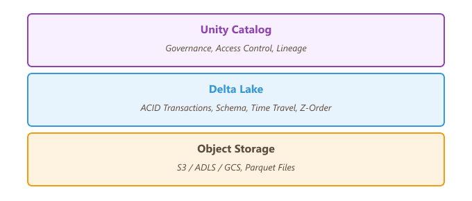
The Lakehouse architecture, popularized by Databricks, layers structured metadata and governance on top of open file formats in object storage. Unlike a traditional data warehouse (which copies data into a proprietary format), the Lakehouse keeps all data in open formats (Parquet via Delta Lake) while providing warehouse features: ACID transactions, indexing, caching, and SQL access.
For LLM teams, the Lakehouse pattern has three practical advantages. First, training data and analytics data live in the same platform, eliminating ETL between systems. Second, the open format means any tool (Spark, pandas, DuckDB, PyArrow) can read the data directly. Third, the governance layer (Unity Catalog) applies consistently across all access patterns, whether a data scientist reads data from a notebook or a training pipeline reads it from a scheduled job.
O.2.6 Optimizing Delta Tables for ML Workloads
Delta Lake includes several optimization features that improve read performance for large training datasets. Z-ordering co-locates related data in the same Parquet files based on column values, which accelerates filtered reads. Compaction (the OPTIMIZE command) merges small files into larger ones, reducing the overhead of reading thousands of tiny files. Liquid clustering, a newer feature, automatically manages data layout without manual Z-order specifications.
-- Compact small files into larger ones (target ~1 GB per file)
OPTIMIZE delta.`s3://bucket/delta/instruction_pairs`;

-- Z-order by columns commonly used for filtering
OPTIMIZE delta.`s3://bucket/delta/instruction_pairs`
  ZORDER BY (source, quality_score);

-- Enable liquid clustering on a new table (Databricks Runtime 13.3+)
CREATE TABLE ml_catalog.llm_data.embeddings (
  doc_id BIGINT,
  chunk_id INT,
  embedding ARRAY<FLOAT>,
  source STRING,
  created_at TIMESTAMP
)
USING DELTA
CLUSTER BY (source, created_at);

-- Vacuum old files (default retention: 7 days)
VACUUM delta.`s3://bucket/delta/instruction_pairs` RETAIN 168 HOURS;The VACUUM command permanently deletes old Parquet files that are no longer referenced by the Delta log. After vacuuming, time travel queries to versions older than the retention period will fail. Always set the retention period longer than your longest-running training job, and keep MLflow logs that record the exact Delta version used for each training run.
Summary
Delta Lake transforms raw object storage into a reliable, versioned data platform suitable for production ML. ACID transactions prevent data corruption during concurrent reads and writes, time travel enables reproducible training by pinning exact dataset versions, and schema enforcement catches upstream data drift before it reaches your model. Combined with Unity Catalog's governance layer, the Lakehouse architecture provides a single source of truth for both analytics and ML workloads. In the next section, we explore Ray, which complements Databricks by providing distributed compute for training and serving workloads that extend beyond Spark's data-parallel paradigm.
Feature Stores for ML
Feature stores solve the "training-serving skew" problem by providing a single system that manages feature computation, storage, and retrieval for both training and inference. In LLM applications, features include user embeddings, document metadata, retrieval scores, and contextual signals that augment prompts or drive routing logic. This section covers three leading feature store platforms: Feast (open source), Tecton (managed), and Databricks Feature Engineering (integrated with Unity Catalog from this section).
O.6.1 The Training-Serving Skew Problem
When building ML-powered applications, features computed during training must match exactly the features available at inference time. Without a feature store, teams often end up with two separate codebases: a batch pipeline (Python/Spark) that computes features for training, and a real-time service (Java/Go) that computes the same features for inference. Subtle differences between these implementations, such as different timestamp handling, rounding behavior, or null treatment, create training-serving skew that silently degrades model performance.
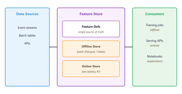
Feature stores address this by defining features once and serving them consistently across both contexts. A feature definition specifies the computation logic, the data source, and the freshness requirements. The feature store then materializes these features into an offline store (for training) and an online store (for low-latency inference), guaranteeing consistency.
O.6.2 Feast: Open-Source Feature Store
Feast is the most widely adopted open-source feature store. It provides a Python SDK for defining features, materializing them from batch or streaming sources into online stores (Redis, DynamoDB, or SQLite for development), and retrieving them with point-in-time correctness for training. Feast integrates with data warehouses like BigQuery, Snowflake, and Redshift as offline stores, and with Delta Lake tables for Databricks environments.
# feature_repo/feature_definitions.py
from datetime import timedelta
from feast import Entity, Feature, FeatureView, FileSource, ValueType
from feast.types import Float32, Int64, String

# Define the entity (the primary key for feature lookups)
user = Entity(
    name="user_id",
    value_type=ValueType.STRING,
    description="Unique user identifier",
)

# Define a data source (Parquet file, BigQuery table, etc.)
user_features_source = FileSource(
    path="s3://bucket/features/user_stats.parquet",
    timestamp_field="event_timestamp",
    created_timestamp_column="created_at",
)

# Define a feature view (a group of related features)
user_features = FeatureView(
    name="user_features",
    entities=[user],
    ttl=timedelta(days=7),  # Features older than 7 days are stale
    schema=[
        Feature(name="total_conversations", dtype=Int64),
        Feature(name="avg_response_rating", dtype=Float32),
        Feature(name="preferred_language", dtype=String),
        Feature(name="user_embedding", dtype=Float32),
    ],
    source=user_features_source,
    online=True,  # Materialize to online store
)# Initialize the Feast feature repository
feast init feature_repo
cd feature_repo
# Apply feature definitions to the registry
feast apply
# Materialize features from offline to online store
feast materialize 2024-01-01T00:00:00 2025-04-01T00:00:00
# Start a local feature server for online serving
feast serve --port 6566For LLM applications, the most common Feast use case is serving user context at inference time. When a user sends a message, your application fetches their feature vector (conversation history length, preferred response style, topic preferences) from the online store and includes it in the system prompt. This personalizes the LLM response without any model fine-tuning.
O.6.3 Point-in-Time Joins for Training
One of the most valuable features of a feature store is point-in-time correct joins.
When building a training dataset, you need to know the value of each feature as it existed at the
time of the training event, not the current value. For example, if a user had 10 conversations when
a particular interaction occurred but now has 500, the training data should reflect the value 10.
Feast handles this automatically through its get_historical_features API.
from feast import FeatureStore
import pandas as pd

store = FeatureStore(repo_path="feature_repo/")

# Entity DataFrame: the events you want to enrich with features
entity_df = pd.DataFrame({
    "user_id": ["user_001", "user_002", "user_003", "user_001"],
    "event_timestamp": pd.to_datetime([
        "2025-01-15 10:00:00",
        "2025-01-15 11:30:00",
        "2025-02-01 09:00:00",
        "2025-03-01 14:00:00",  # Same user, different time
    ]),
})

# Fetch features with point-in-time correctness
training_df = store.get_historical_features(
    entity_df=entity_df,
    features=[
        "user_features:total_conversations",
        "user_features:avg_response_rating",
        "user_features:preferred_language",
    ],
).to_df()

print(training_df)
# user_001 at Jan 15 gets their Jan 15 feature values
# user_001 at Mar 01 gets their Mar 01 feature values (different!)O.6.4 Tecton: Managed Feature Platform
Tecton is a managed feature platform built by the team that created Feast at Uber. It extends the feature store concept with a feature pipeline engine that handles both batch and real-time feature computation. Unlike Feast, which requires you to compute features externally and point to the results, Tecton defines the transformation logic alongside the feature definition and orchestrates the computation automatically. Tecton is available as a managed service and integrates with Databricks, Snowflake, and Spark.
# Tecton feature definition with built-in transformation
from tecton import Entity, BatchSource, batch_feature_view
from tecton.types import Field, String, Float64, Int64
from datetime import timedelta

# Entity definition
user = Entity(name="user", join_keys=["user_id"])

# Batch feature view with transformation logic
@batch_feature_view(
    sources=[conversation_logs_source],
    entities=[user],
    mode="spark_sql",
    batch_schedule=timedelta(days=1),
    ttl=timedelta(days=30),
    online=True,
    offline=True,
    feature_start_time="2024-01-01",
    schema=[
        Field("user_id", String),
        Field("total_conversations", Int64),
        Field("avg_response_length", Float64),
        Field("avg_quality_rating", Float64),
    ],
)
def user_conversation_stats(conversation_logs):
    return f"""
        SELECT
            user_id,
            COUNT(*) as total_conversations,
            AVG(response_length) as avg_response_length,
            AVG(quality_rating) as avg_quality_rating
        FROM {conversation_logs}
        GROUP BY user_id
"""The key difference between Feast and Tecton is where the computation happens. Feast is a "feature serving" layer: you compute features externally and register the results. Tecton is a "feature platform" that also manages computation. For teams that already have robust data pipelines (perhaps using Databricks or Airflow), Feast provides the serving layer without duplicating orchestration. For teams building from scratch, Tecton's integrated computation reduces the number of systems to manage.
O.6.5 Databricks Feature Engineering
Databricks provides its own feature engineering capabilities through the databricks-feature-engineering
SDK, tightly integrated with Unity Catalog (see this section). Feature
tables are standard Delta tables with additional metadata that marks specific columns as features and
one or more columns as the lookup key. The advantage of this approach is that feature governance,
lineage, and access control are inherited directly from Unity Catalog.
from databricks.feature_engineering import FeatureEngineeringClient, FeatureLookup

fe = FeatureEngineeringClient()

# Create a feature table from a Spark DataFrame
user_features_df = spark.sql("""
    SELECT
        user_id,
        COUNT(*) as total_conversations,
        AVG(response_rating) as avg_response_rating,
        COLLECT_LIST(topic) as topic_history
    FROM ml_catalog.llm_data.conversations
    GROUP BY user_id
""")

fe.create_table(
    name="ml_catalog.features.user_conversation_stats",
    primary_keys=["user_id"],
    df=user_features_df,
    description="Aggregated conversation statistics per user",
)

# Create a training dataset with automatic feature lookup
training_events = spark.read.table("ml_catalog.llm_data.training_events")

training_set = fe.create_training_set(
    df=training_events,
    feature_lookups=[
        FeatureLookup(
            table_name="ml_catalog.features.user_conversation_stats",
            lookup_key=["user_id"],
            feature_names=["total_conversations", "avg_response_rating"],
        ),
    ],
    label="quality_label",
)

training_df = training_set.load_df()
print(f"Training set with features: {training_df.columns}")O.6.6 Choosing a Feature Store for LLM Applications
The right feature store depends on your existing infrastructure and the complexity of your feature pipelines. The table below summarizes the tradeoffs for each platform.
| Criterion | Feast | Tecton | Databricks FE |
|---|---|---|---|
| Deployment | Self-hosted (open source) | Managed SaaS | Integrated with Databricks |
| Feature computation | External (bring your own) | Built-in (Spark, Rift) | Spark notebooks/jobs |
| Online store options | Redis, DynamoDB, SQLite | DynamoDB, Redis | Databricks Online Tables |
| Streaming features | Via push sources | Native (Spark Streaming) | Via Delta Live Tables |
| Governance | Manual | Built-in RBAC | Unity Catalog |
| Best for | Teams with existing pipelines | Greenfield ML platforms | Databricks-centric orgs |
Feature stores add operational complexity. If your LLM application only uses prompt-time context (retrieved documents, conversation history) without computed features, you may not need a feature store at all. Adopt one when you find yourself maintaining duplicate feature computation logic between training and serving, or when feature freshness and consistency become reliability risks.
Summary
Feature stores bridge the gap between training and serving by providing a single source of truth for computed features. Feast offers an open-source, bring-your-own-compute approach that integrates with any data stack. Tecton provides a managed platform with built-in feature computation and orchestration. Databricks Feature Engineering leverages Unity Catalog for governance and integrates seamlessly with the broader Databricks ecosystem. For LLM applications, feature stores are most valuable when your system uses computed user or document features alongside retrieval-augmented generation. In the next section, we bring all these components together into production data pipelines and model serving architectures at scale.
What's Next?
In the next section, Section 19.5: Models, we build on the material covered here.