There are only two hard problems in computer science: cache invalidation, naming things, and choosing a vector database.
Vec, Humorously Pedantic AI Agent
A vector database is more than an ANN index with an API. Production vector search requires persistent storage, metadata filtering, access control, horizontal scaling, real-time updates, and monitoring. The vector database ecosystem has expanded rapidly, offering options that range from fully managed cloud services to embedded libraries that run in-process. Choosing the right solution depends on your scale, infrastructure, operational maturity, and whether you need features like hybrid search, multi-tenancy, or built-in reranking. Building on the ANN algorithms from Section 31.3, this section provides a practical, comparative guide to the major systems.
Prerequisites
This section assumes you understand the vector index algorithms (HNSW, IVF, PQ) from Section 31.3 and the embedding model landscape from Section 31.1. Experience with database systems or cloud infrastructure will help you evaluate the operational tradeoffs between managed and self-hosted solutions.

31.5.1 Vector Database Architecture
A team upgraded their embedding model from text-embedding-ada-002 to text-embedding-3-small for a 60% cost reduction. They re-indexed the corpus. Within a week, retrieval-quality complaints spiked 4×: queries returning unrelated documents. Root cause: they had embedded the corpus with the new model but the production query path still loaded a cached query-embedding model that used the OLD weights. New corpus vectors and old query vectors lived in different embedding spaces; cosine similarity between them was meaningless. Fix: explicit version tag on every index entry; on query, verify embedding-model version matches index version, fail loudly if not. Lesson: embedding-model upgrades require atomic switchover of BOTH the indexer AND the query encoder, with a regression eval in between.
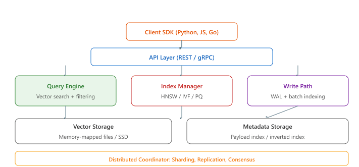
A vector database extends the ANN index algorithms covered in Section 31.3 with the operational features needed for production deployments. The core architectural components are listed below.
- Storage engine: Persists vectors and metadata to disk with write-ahead logging for durability. Must support efficient bulk loading and incremental updates.
- Index manager: Builds and maintains ANN indexes (HNSW, IVF, etc.), handles index rebuilds, and manages index parameters.
- Query engine: Processes search requests, combining vector similarity with metadata filters and optional reranking.
- API layer: Exposes gRPC and/or REST endpoints for CRUD operations, search, and administration.
- Distributed coordinator: (For distributed systems) Manages sharding, replication, consistency, and load balancing across nodes.
FAISS, Annoy, and ScaNN are vector index libraries, not databases. They provide fast approximate nearest neighbor search but lack persistence, metadata filtering, access control, real-time updates, and horizontal scaling. Using FAISS in production without wrapping it in a proper storage and serving layer means you lose data on restart, cannot filter by metadata, and cannot update individual vectors without rebuilding the entire index. A vector database (Pinecone, Qdrant, Weaviate, Milvus) wraps an ANN index with the operational features needed for production workloads. Choose a library for prototyping or embedded use cases; choose a database when you need durability, filtering, and multi-user access.
31.5.2 Purpose-Built Vector Databases
The distinction between a vector index library and a vector database makes the next question obvious: which production-grade database should you pick? Four serious contenders (Pinecone, Qdrant, Weaviate, Milvus) compete on different axes of managed-vs-self-hosted, metadata filtering, and clustering model. We start with Pinecone because its fully-managed serverless tier is what most teams encounter first.
Pinecone
If you are building a prototype or proof of concept, start with Chroma (in-process, zero infrastructure) or Pinecone serverless (managed, free tier). For production stacks where Postgres is already the system of record, pgvector + Supabase (or AWS RDS / Aurora) has become the dominant SQL-native default in 2025-2026 because it keeps vectors alongside relational data and avoids a second database. Turbopuffer (built on object storage, 2024) is the emerging cost-efficient option for billion-scale archive workloads where read latency tolerates 50-150 ms. Move to self-hosted Qdrant, Weaviate, or LanceDB when you need features like multi-tenancy, custom reranking, or data residency guarantees that managed options cannot provide.
Pinecone is a fully managed, cloud-native vector database. It eliminates operational overhead by handling infrastructure, scaling, and index management automatically. Pinecone provides serverless and pod-based deployment options, with serverless being the more cost-effective choice for workloads with variable traffic patterns. Like the managed LLM APIs covered earlier, managed vector databases trade operational control for faster time to production.
# Pinecone: managed vector database
from pinecone import Pinecone, ServerlessSpec
pc = Pinecone(api_key="your-api-key")
# Create a serverless index
pc.create_index(
    name="document-search",
    dimension=768,
    metric="cosine",
    spec=ServerlessSpec(
    cloud="aws",
    region="us-east-1"
    )
    )
index = pc.Index("document-search")
# Upsert vectors with metadata
vectors = [
    {
    "id": "doc-001",
    "values": [0.12, -0.34, 0.56, ...], # 768-dim embedding
    "metadata": {
    "source": "annual-report-2024.pdf",
    "page": 15,
    "category": "financial",
    "date": "2024-03-15"
    }
    },
    {
    "id": "doc-002",
    "values": [0.45, 0.23, -0.78, ...],
    "metadata": {
    "source": "product-manual.pdf",
    "page": 42,
    "category": "technical",
    "date": "2024-01-20"
    }
    }
    ]
index.upsert(vectors=vectors)
# Search with metadata filtering
results = index.query(
    vector=[0.11, -0.32, 0.54, ...],
    top_k=5,
    filter={
    "category": {"$eq": "financial"},
    "date": {"$gte": "2024-01-01"}
    },
    include_metadata=True
    )
for match in results["matches"]:
    print(f"Score: {match['score']:.4f}, "
        f"Source: {match['metadata']['source']}, "
f"Page: {match['metadata']['page']}")The vector database market went from "what's a vector database?" to over a dozen funded startups in roughly 18 months (2022 to 2024). For a brief period, adding "vector" to your database's name was the fastest way to raise a Series A.
Qdrant
Qdrant is an open-source vector database written in Rust, designed for high performance and operational flexibility. It supports both self-hosted and cloud-managed deployments. Qdrant's key differentiators include rich payload filtering with indexed fields, built-in support for sparse vectors (enabling hybrid search natively), and quantization options (scalar, product, and binary) for memory optimization.
# Qdrant: high-performance open-source vector database
from qdrant_client import QdrantClient
from qdrant_client.models import (
    Distance, VectorParams, PointStruct,
    Filter, FieldCondition, MatchValue,
    NamedVector, SparseVector, SparseVectorParams,
    SparseIndexParams,
    )
client = QdrantClient(url="http://localhost:6333")
# Create collection with both dense and sparse vectors (hybrid search)
client.create_collection(
    collection_name="documents",
    vectors_config={
    "dense": VectorParams(size=768, distance=Distance.COSINE),
    },
    sparse_vectors_config={
    "sparse": SparseVectorParams(
    index=SparseIndexParams(on_disk=False)
    ),
    },
    )
# Upsert points with dense vectors, sparse vectors, and payload
client.upsert(
    collection_name="documents",
    points=[
    PointStruct(
    id=1,
    vector={
    "dense": [0.12, -0.34, 0.56] + [0.0] * 765,
    "sparse": SparseVector(
    indices=[102, 507, 1024, 3891],
    values=[0.8, 0.6, 0.9, 0.3]
    ),
    },
    payload={
    "title": "Introduction to RAG Systems",
    "category": "technical",
    "word_count": 2500,
    },
    ),
    ],
    )
# Hybrid search: combine dense and sparse retrieval
results = client.query_points(
    collection_name="documents",
    prefetch=[
    # Dense vector search
    {"query": [0.11, -0.32, 0.54] + [0.0] * 765, "using": "dense", "limit": 20},
    # Sparse vector search (BM25-style)
    {"query": SparseVector(indices=[102, 1024], values=[0.9, 0.7]),
    "using": "sparse", "limit": 20},
    ],
    # Reciprocal Rank Fusion to merge results
    query={"fusion": "rrf"},
    limit=10,
    )
for point in results.points:
print(f"ID: {point.id}, Score: {point.score:.4f}")Weaviate
Weaviate is an open-source vector database that integrates embedding generation directly into its query pipeline. Through its module system, Weaviate can automatically vectorize text at ingestion and query time using built-in integrations with OpenAI, Cohere, Hugging Face, and other providers. This simplifies the development workflow by eliminating the need to manage embedding generation separately.
Milvus
Milvus is an open-source distributed vector database designed for billion-scale workloads. Its disaggregated architecture separates storage and compute, allowing independent scaling of query nodes, data nodes, and index nodes. Milvus supports the widest range of index types (HNSW, IVF-Flat, IVF-PQ, IVF-SQ8, DiskANN, GPU indexes) and provides strong consistency guarantees through a log-based architecture.
31.5.3 Lightweight and Embedded Solutions
Milvus and the other purpose-built systems target billion-vector workloads, which is overkill for a tutorial, a research notebook, or a small application. The lighter tier (Chroma, LanceDB, SQLite-vss) trades multi-region replication for zero-infrastructure embedded use. We start with ChromaDB, which has become the canonical default for prototyping.
ChromaDB
ChromaDB is an open-source embedding database designed for simplicity and rapid prototyping. It runs in-process (embedded mode) or as a lightweight server, making it the most popular choice for local development, tutorials, and small-scale applications. ChromaDB handles embedding generation automatically when configured with an embedding function.
# ChromaDB: lightweight embedded vector database
import chromadb
from chromadb.utils.embedding_functions import SentenceTransformerEmbeddingFunction
# Initialize with persistent storage
client = chromadb.PersistentClient(path="./chroma_data")
# Use Sentence Transformers for automatic embedding
embedding_fn = SentenceTransformerEmbeddingFunction(
    model_name="all-MiniLM-L6-v2"
    )
# Create or get collection
collection = client.get_or_create_collection(
    name="knowledge_base",
    embedding_function=embedding_fn,
    metadata={"hnsw:space": "cosine"}
    )
# Add documents (embeddings generated automatically)
collection.add(
    documents=[
    "RAG combines retrieval with language model generation.",
    "Vector databases store and index high-dimensional embeddings.",
    "HNSW provides fast approximate nearest neighbor search.",
    "Chunking strategies affect retrieval quality significantly.",
    ],
    metadatas=[
    {"topic": "rag", "level": "intro"},
    {"topic": "vector-db", "level": "intro"},
    {"topic": "algorithms", "level": "advanced"},
    {"topic": "preprocessing", "level": "intermediate"},
    ],
    ids=["doc1", "doc2", "doc3", "doc4"]
    )
# Query with automatic embedding and metadata filtering
results = collection.query(
    query_texts=["How does semantic search work?"],
    n_results=3,
    where={"level": {"$ne": "advanced"}}
    )
for doc, distance, metadata in zip(
    results["documents"][0],
    results["distances"][0],
    results["metadatas"][0]
    ):
print(f"Distance: {distance:.4f} | {metadata['topic']}: {doc[:60]}...")The chromadb package (v0.5+, 2024 to 2026) is the smallest functional vector DB: zero servers, one PersistentClient call, and you have HNSW indexing, metadata filtering, and an automatic embedding pipeline on disk. Use it for prototypes, evaluation harnesses, and laptops; graduate to Qdrant or pgvector once you need horizontal scaling or transactional consistency.
Show code
pip install chromadb
import chromadb

client = chromadb.PersistentClient(path="./chroma_data")
col = client.get_or_create_collection(
    name="kb", metadata={"hnsw:space": "cosine"}
)
col.add(
    ids=["d1", "d2"],
    documents=["RAG retrieves then generates.", "HNSW gives sub-ms search."],
    metadatas=[{"src": "wiki"}, {"src": "blog"}],
)
hits = col.query(query_texts=["how does retrieval work?"], n_results=2)FAISS as a Library
FAISS (Facebook AI Similarity Search) is not a database but a library for building and querying ANN indexes. It provides the fastest index implementations available, with GPU acceleration for both index building and search. FAISS is the right choice when you need maximum search performance, have a static or infrequently updated dataset, and are willing to handle persistence and metadata filtering yourself.
LanceDB
LanceDB is a serverless, embedded vector database built on the Lance columnar format. Its distinguishing feature is storing vectors alongside structured data in a single table, much like a traditional database that happens to support vector search. LanceDB supports automatic versioning of data, zero-copy access through memory-mapped files, and integration with the broader data ecosystem through Apache Arrow compatibility.
pgvector
pgvector is a PostgreSQL extension that adds vector similarity search capabilities to the world's most popular open-source relational database. For teams already running PostgreSQL, pgvector eliminates the need to introduce and operate a separate vector database. It supports HNSW and IVF-Flat indexes and benefits from PostgreSQL's mature ecosystem of tooling, replication, and backup solutions.
# pgvector: vector search in PostgreSQL
import psycopg2
import numpy as np
conn = psycopg2.connect("postgresql://user:pass@localhost/mydb")
cur = conn.cursor()
# Enable the extension and create table
cur.execute("CREATE EXTENSION IF NOT EXISTS vector;")
cur.execute("""
    CREATE TABLE IF NOT EXISTS documents (
    id SERIAL PRIMARY KEY,
    content TEXT,
    category TEXT,
    embedding vector(768)
    );
    """)
# Create HNSW index for cosine distance
cur.execute("""
    CREATE INDEX IF NOT EXISTS documents_embedding_idx
    ON documents
    USING hnsw (embedding vector_cosine_ops)
    WITH (m = 16, ef_construction = 200);
    """)
# Insert documents with embeddings
sample_embedding = np.random.randn(768).astype(np.float32)
sample_embedding /= np.linalg.norm(sample_embedding)
cur.execute(
    """INSERT INTO documents (content, category, embedding)
    VALUES (%s, %s, %s)""",
    ("Vector databases enable semantic search.", "technical",
    sample_embedding.tolist())
    )
conn.commit()
# Semantic search with SQL: combine vector similarity with standard filters
query_embedding = np.random.randn(768).astype(np.float32)
query_embedding /= np.linalg.norm(query_embedding)
cur.execute("""
    SELECT id, content, category,
    1 - (embedding <=> %s::vector) AS similarity
    FROM documents
    WHERE category = 'technical'
    ORDER BY embedding <=> %s::vector
    LIMIT 5;
    """, (query_embedding.tolist(), query_embedding.tolist()))
for row in cur.fetchall():
    print(f"ID: {row[0]}, Similarity: {row[3]:.4f}, Content: {row[1][:50]}...")
    cur.close()
conn.close()pgvector is an excellent choice when: (1) you already operate PostgreSQL and want to minimize infrastructure complexity; (2) your vector collection is under 10 million items; (3) you need transactional consistency between vector data and relational data; or (4) your queries combine vector similarity with complex SQL filters and joins. For collections above 10 million vectors or workloads requiring sub-millisecond latency at scale, a purpose-built vector database will generally outperform pgvector.
31.5.4 Comparison Matrix
| System | Type | Language | Managed Cloud | Hybrid Search | Best For |
|---|---|---|---|---|---|
| Pinecone | Managed DB | N/A (SaaS) | Yes (only) | Yes | Zero-ops production |
| Qdrant | Open-source DB | Rust | Yes | Yes (native) | High performance, flexibility |
| Weaviate | Open-source DB | Go | Yes | Yes | Built-in vectorization |
| Milvus | Open-source DB | Go/C++ | Yes (Zilliz) | Yes | Billion-scale distributed |
| ChromaDB | Embedded DB | Python | No | No | Prototyping, small scale |
| FAISS | Library | C++/Python | No | No | Maximum raw performance |
| LanceDB | Embedded DB | Rust | Yes | Yes | Data-native workflows |
| pgvector | Extension | C | Via PG hosts | Via SQL | Existing PostgreSQL stacks |
31.5.5 Metadata Filtering

Real-world retrieval rarely uses pure vector similarity. Most queries include metadata constraints such as date ranges, document categories, access permissions, or language filters. The efficiency of metadata filtering varies significantly across systems.
Pre-filtering vs. Post-filtering
- Pre-filtering: Apply metadata filters first, then search only within the matching subset. This is efficient when the filter is highly selective (eliminates most vectors) but can degrade ANN quality if the filtered subset is small relative to the index structure.
- Post-filtering: Perform the ANN search first, then remove results that do not match the metadata filter. This preserves ANN quality but may return fewer results than requested if many top results are filtered out.
- Integrated filtering: The most sophisticated approach interleaves filtering with the ANN search algorithm. Qdrant and Weaviate implement this by checking metadata predicates during graph traversal, combining the benefits of both approaches.
Metadata filtering can silently degrade retrieval quality. If your filter eliminates 99% of vectors and you are using post-filtering, a search for top-10 results might return only 1 or 2 matches. If you are using pre-filtering with an HNSW index built on the full dataset, the search may miss relevant results because the graph connectivity has been disrupted. Always monitor the number of results returned and the score distribution to detect filtering-related quality issues.
31.5.6 Hybrid Search and Reciprocal Rank Fusion
Hybrid search combines dense vector retrieval (semantic similarity) with sparse keyword retrieval (lexical matching, typically BM25). This addresses a fundamental limitation of pure semantic search: embedding models may miss exact keyword matches that are critical for some queries, especially those involving proper nouns, product codes, or technical terminology.
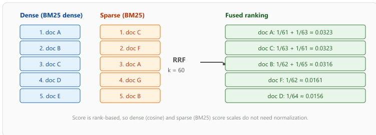
Reciprocal Rank Fusion (RRF)
RRF is the most common method for merging ranked result lists from different retrieval systems.
For each document, RRF computes a fused score based on its rank position in each result list,
using the formula: score = sum(1 / (k + rank_i)), where k is a constant
(typically 60) and rank_i is the document's position in the i-th result list.
Documents that appear near the top of multiple lists receive the highest fused scores.
Formally, given $R$ ranked lists from $R$ retrievers and a document $d$ that appears at rank $\mathrm{rank}_i(d)$ in list $i$ (with $1/(k + \infty) = 0$ if $d$ is absent), the fused score is:
Cormack et al. (2009) recommend $k = 60$. The constant flattens the contribution of top-1 vs. top-2 vs. top-3 results so that an early-rank disagreement between retrievers does not dominate; the asymptotic $1/\mathrm{rank}$ shape still rewards documents seen near the top of multiple lists.
# Reciprocal Rank Fusion implementation
from typing import Dict, List, Tuple
def reciprocal_rank_fusion(
    result_lists: List[List[str]],
    k: int = 60
    ) -> List[Tuple[str, float]]:
    """
                                                                                                                                                                                                                                                                                                                                                                                                                                                                                                                                                                                                                                                                                                                                                                                                                                    Merge multiple ranked result lists using RRF.
    Args:
    result_lists: List of ranked document ID lists
    k: RRF constant (default 60, as per the original paper)
    Returns:
    List of (doc_id, fused_score) tuples, sorted by fused score
    """
    fused_scores: Dict[str, float] = {}
    for result_list in result_lists:
        for rank, doc_id in enumerate(result_list, start=1):
            if doc_id not in fused_scores:
                fused_scores[doc_id] = 0.0
                fused_scores[doc_id] += 1.0 / (k + rank)
                # Sort by fused score descending
                sorted_results = sorted(
                    fused_scores.items(),
                    key=lambda x: x[1],
                    reverse=True
                    )
                return sorted_results
# Example: merge dense and sparse retrieval results
dense_results = ["doc_A", "doc_B", "doc_C", "doc_D", "doc_E"]
sparse_results = ["doc_C", "doc_F", "doc_A", "doc_G", "doc_B"]
fused = reciprocal_rank_fusion([dense_results, sparse_results])
print("Hybrid search results (RRF):")
for doc_id, score in fused[:5]:
print(f" {doc_id}: {score:.6f}")Hybrid search provides the largest improvement over pure dense retrieval when queries contain specific entities (company names, product IDs, error codes) or when the embedding model was not trained on your domain vocabulary. In benchmarks, hybrid search with RRF typically improves recall@10 by 5 to 15% over dense-only retrieval. The improvement is smallest for broad, conceptual queries where semantic matching already excels.
31.5.7 Operational Considerations
Picking a database and tuning hybrid search gets you a working system; keeping it working as the corpus grows is a separate discipline. Three operational levers dominate: how you scale (vertically, by sharding, or by tiering), how you back up and recover, and how you observe latency and recall in production. We start with the scaling patterns because they shape every other decision.
Scaling Patterns
- Vertical scaling: Add more RAM and faster CPUs to a single node. This is the simplest approach and works well up to approximately 10 to 50 million vectors, depending on dimensionality and quantization.
- Sharding: Distribute vectors across multiple nodes based on a partition key. Each shard handles a subset of the data. Queries are fanned out to all shards and results are merged.
- Replication: Copy each shard to multiple nodes for fault tolerance and read throughput. Read queries can be load-balanced across replicas.
Cost Optimization
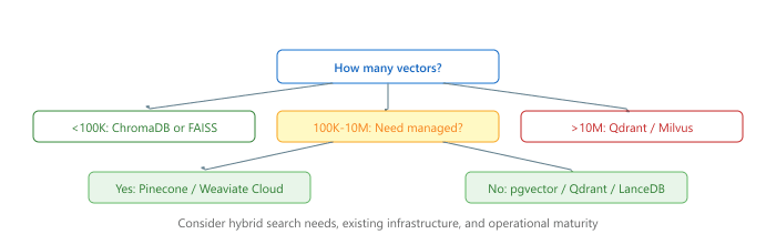
Vector databases can become expensive at scale because they require significant memory. Key strategies for cost reduction include: using quantization (scalar, product, or binary) to reduce memory per vector; using disk-based indexes (DiskANN) for cold data; implementing tiered storage where frequently accessed data stays in memory while archival data resides on SSD; and choosing serverless pricing models that scale to zero during idle periods. Figure 31.5.5c provides a decision tree to guide this selection.
Combine vector similarity search with metadata pre-filtering (by date, source, category) to dramatically improve relevance. Searching 1,000 pre-filtered documents is faster and more accurate than searching 1 million and hoping the embeddings capture the right context.
Who: A backend engineer at a B2B SaaS company providing AI-powered customer support
Situation: The team initially stored 500K support ticket embeddings in PostgreSQL with pgvector, which kept the stack simple since they already ran Postgres for transactional data.
Problem: As the dataset grew to 8 million vectors across 200 tenants, pgvector queries slowed to 400ms at the 95th percentile. Index rebuilds after bulk ingestion locked the table for minutes, causing downtime.
Dilemma: Switching to Pinecone would solve performance issues with fully managed scaling, but at $0.096 per million vectors per hour the annual cost would reach $67K. Weaviate (self-hosted) was cheaper but required the team to manage Kubernetes clusters and handle replication themselves.
Decision: They migrated to self-hosted Qdrant on Kubernetes, which offered tenant isolation via collection-level namespaces, native HNSW indexing, and a straightforward operational model.
How: They ran a parallel-write migration over two weeks, writing to both pgvector and Qdrant, then cut over after validating recall parity on 10,000 test queries.
Result: P95 latency dropped to 25ms, bulk ingestion no longer caused downtime, and infrastructure costs stayed under $18K annually on three dedicated nodes.
Lesson: pgvector is excellent for prototyping and small datasets, but dedicated vector databases become necessary when multi-tenancy, scale, or uptime requirements exceed what a relational add-on can deliver.
Disaggregated vector search separates compute from storage, allowing index serving to scale independently of data ingestion. Multi-modal vector databases are extending beyond text to natively support image, audio, and video embeddings with cross-modal search capabilities. Serverless vector databases (e.g., Pinecone Serverless, Qdrant Cloud) are reducing the operational burden by scaling to zero when idle and auto-scaling under load. Research into filtered vector search is improving the efficiency of combining metadata filters with approximate nearest neighbor queries, a persistent pain point in production RAG systems where users need to scope searches by date, source, or category.
- Vector databases add production features (persistence, filtering, scaling, APIs) on top of ANN algorithms, going well beyond raw index performance.
- Pinecone offers zero-ops managed service; Qdrant and Milvus provide high-performance open-source alternatives with cloud options.
- ChromaDB is ideal for prototyping and small-scale applications; FAISS delivers maximum raw performance as a library.
- pgvector is the pragmatic choice for teams already running PostgreSQL with collections under 10M vectors.
- Metadata filtering strategy (pre-filter, post-filter, or integrated) significantly affects both result quality and query latency.
- Hybrid search with RRF typically improves recall by 5 to 15% over dense-only retrieval, especially for entity-rich queries.
- Start simple, scale up. Begin with ChromaDB or pgvector for prototyping, then migrate to a purpose-built solution when scale or feature requirements demand it.
Show Answer
Show Answer
Show Answer
Show Answer
Show Answer
Exercises
You have 50,000 documents that rarely change and need semantic search. Would you use Pinecone, Qdrant, or ChromaDB? Justify your choice.
Show Answer
ChromaDB is ideal for this scale: it runs embedded (no server needed), supports 50K vectors easily in memory, and is simple to set up. Pinecone would be overkill (and costs money), while Qdrant would work but requires running a server for a small dataset.
Explain the difference between pre-filtering and post-filtering in vector search. When does pre-filtering hurt recall, and how can you mitigate this?
Show Answer
Pre-filtering removes vectors before ANN search, which can eliminate relevant vectors from clusters. Post-filtering runs ANN first, then filters results, which may return fewer than K results. Mitigation: over-fetch (retrieve 3 to 5x K) then post-filter, or use indexes that support native filtering.
Describe how Reciprocal Rank Fusion (RRF) combines dense and sparse search results. Why is it preferred over simple score normalization?
Show Answer
RRF scores each result as 1/(k + rank) and sums across retrievers. It is rank-based, so it avoids the problem of incompatible score scales between dense (cosine similarity) and sparse (BM25) systems. Score normalization requires knowing the min/max of each scorer, which is fragile.
Your vector database currently holds 10 million vectors and handles 100 QPS. Traffic is expected to grow to 1000 QPS. What scaling strategies would you consider?
Show Answer
Options: (a) read replicas for horizontal scaling of queries, (b) sharding the index across multiple nodes, (c) caching frequent queries, (d) upgrading to a larger instance. Start with read replicas as the simplest option.
Compare namespace isolation vs. metadata-based tenant filtering for a multi-tenant vector search application. What are the security and performance implications of each approach?
Show Answer
Namespace isolation: each tenant gets a separate collection/namespace. Stronger security (no cross-tenant leakage), simpler permission model, but more resource overhead. Metadata filtering: all tenants share one collection with a tenant_id field. More efficient resource usage, but requires careful filter enforcement and risks cross-tenant exposure if filters are bypassed.
Create a ChromaDB collection, insert 100 text chunks with metadata (source, date), and perform a filtered search that retrieves only documents from a specific source.
Implement Reciprocal Rank Fusion that combines results from a BM25 search and a dense vector search. Test on a dataset of 1000 documents and compare recall against each method alone.
Set up both Qdrant (via Docker) and ChromaDB with the same dataset of 100,000 embeddings. Compare insertion throughput, query latency at various batch sizes, and memory usage.
What Comes Next
In the next section, Section 31.6: Document Processing & Chunking, we cover document processing and chunking strategies, the critical preprocessing step that determines retrieval quality.