You shall know a word by the company it keeps.
Vec, Linguistically Social AI Agent
Section 31.1 covered the classical lineage: bi-encoder vs. cross-encoder, mean pooling, contrastive learning with InfoNCE, and hard-negative mining. This section picks up where that left off and surveys the 2022-26 wave of embedding innovations: Matryoshka representation learning (nestable dimensions), ColBERT-style late interaction (per-token retrieval), instruction-tuned and asymmetric retrieval embeddings (E5, BGE, GTE, Nomic, Jina), MTEB-driven model selection, and the practical realities (query/passage prefixing, geometry, fine-tuning, production tradeoffs) that decide which model ships.
Prerequisites
This section assumes the bi-encoder versus cross-encoder discussion from Section 31.1, the embedding-model fundamentals from Section 3.1, and the BERT-style encoder architecture from Section 5.1. Familiarity with the contrastive-learning objective from Section 3.6 will help you read the loss-function discussions.
31.2.1 Modern Embedding Architectures
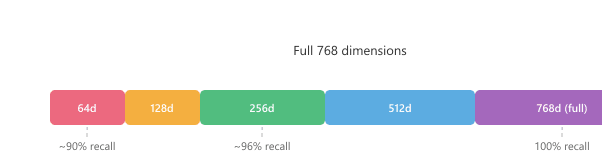
Matryoshka Representation Learning is named after Russian nesting dolls because each prefix of the embedding vector is itself a valid embedding, just smaller. The trick has the delightful property that a single trained model gives you 32-dim, 64-dim, 128-dim, and 768-dim embeddings for free, which sounds suspicious until you realize it works because you train it that way. Kusupati et al. published it in 2022; OpenAI shipped it in text-embedding-3 a year later, and now every serious embedding vendor has a "dimensions" knob in the API.
Matryoshka Representation Learning (MRL)
Traditional embedding models produce fixed-dimension vectors (e.g., 768 or 1536 dimensions). If you need smaller vectors for storage efficiency, you must train a separate model. Matryoshka Representation Learning (Kusupati et al., 2022) solves this by training a single model whose embeddings are useful at multiple dimensionalities. The first d dimensions of a 768-dimensional embedding form a valid d-dimensional embedding, much like nested Russian dolls.
During training, the loss function is computed at multiple truncation points (e.g., dimensions 32, 64, 128, 256, 512, 768), and the gradients from all truncation levels are summed. This forces the model to pack the most important information into the leading dimensions. Figure 31.2.1 visualizes this nested structure.
Algorithm: MRL contrastive training
Input:  encoder f_theta producing full-dim embeddings z = f_theta(x) in R^d
        set of nested dimensionalities M = {d_1 < d_2 < ... < d_K = d}
        loss family L(.) (e.g., InfoNCE for retrieval, cross-entropy for classification)
        per-level weights w_1, .., w_K (typically uniform, sum to 1)
Output: encoder whose first d_m coordinates form a valid d_m-embedding for every m

  // For every minibatch (x, x_pos, {x_neg^j})
  z      := f_theta(x)
  z_pos  := f_theta(x_pos)
  z_neg  := f_theta(x_neg^j) for j

  L_total := 0
  For m = 1..K:
      // Truncate all three vectors to the first d_m coordinates,
      // re-L2-normalize the truncated vector.
      z_m     := normalize(z[:d_m])
      z_pos_m := normalize(z_pos[:d_m])
      z_neg_m := normalize(z_neg[:d_m])

      L_m := L( z_m, z_pos_m, z_neg_m )                // e.g. InfoNCE
      L_total := L_total + w_m * L_m

  Backprop on L_total; update theta

Effect. Summing the truncated losses forces the network to put the most discriminative
content in the first d_1 coords, the next-most-discriminative in d_1..d_2, and so on.
At inference any d_m can be used by simple slicing + renormalization; no separate
projection head, no re-training.

Practical menu (OpenAI text-embedding-3, Nomic v1.5, BGE-M3):
   d in {64, 128, 256, 512, 768 (or 1024, 1536, 3072)}
   storage savings: d_m / d_K, e.g. 64 / 1536 ~= 4.2 percent of full storage,
retrieval recall at d_m = 64 is typically 85..92 percent of full-dim recall.Source: Kusupati, Bhatt, Rege, Wallingford et al., "Matryoshka Representation Learning," NeurIPS 2022 (arXiv:2205.13147). The 2024 OpenAI text-embedding-3 family and the Nomic/BGE-M3 lines all expose this menu via a single dimensions parameter, which is the production realization of the MRL idea: one trained encoder, many deployment dimensionalities.
The aha: in a normal embedding, every coordinate contributes roughly equally and there is no "important" prefix to truncate to. Matryoshka changes the training loss, not the architecture, so during optimization the network is simultaneously penalized for the contrastive loss at 64-d, 128-d, 256-d, 512-d, and full-d. The only weight configuration that minimizes all five losses is one that crams the most semantic signal into the first 64 coords, the next most into 65-128, and so on. After training you have not five separate models, you have one model whose coordinate axes were forced to be a sorted importance list. Truncation then just keeps the most-informative coords and drops the rest.
ColBERT: Late Interaction
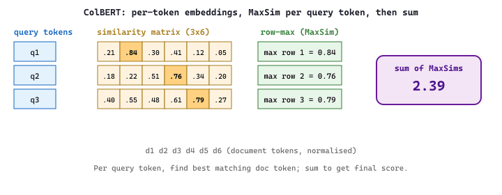
ColBERT introduces a late interaction paradigm that sits between bi-encoders and cross-encoders. Instead of compressing each sentence into a single vector, ColBERT retains per-token embeddings for both the query and the document. At search time, it computes the maximum similarity between each query token and all document tokens (MaxSim), then sums these scores across query tokens.
Formally, given query token embeddings $\{q_1, \dots, q_m\}$ and document token embeddings $\{d_1, \dots, d_n\}$ (both L2-normalised), the ColBERT score is
that is, for every query token pick its most similar document token and sum those maxima. This decomposition is what makes ColBERT a "late" interaction: the per-token embeddings are computed independently (so document side can be precomputed), but the interaction between query and document still happens at the token level, not the sentence level.
This approach preserves much of the expressiveness of cross-encoders while still allowing document token embeddings to be precomputed. The tradeoff is storage: a document with 200 tokens requires storing 200 vectors instead of one. ColBERT v2 addresses this through residual compression, reducing storage by 6 to 10 times while preserving retrieval quality.
Query: "How does GQA reduce KV cache size?". Bi-encoder cosine similarity against passage A (the Llama 3 GQA paragraph) is 0.62, and against passage B (a generic Transformer overview) is 0.61: nearly indistinguishable. ColBERT computes the per-token MaxSim grid: the query token "GQA" maxes at 0.91 in passage A (against the literal "GQA" token) but only 0.18 in passage B (best match is "attention"). Summed over the seven query tokens, passage A scores 4.7 vs passage B's 3.1. The bi-encoder margin of 0.01 becomes a ColBERT margin of 1.6, large enough to robustly retrieve A. This is the kind of "needle-in-paraphrase" failure that motivates late interaction whenever exact-term match still matters.
# ColBERT-style MaxSim scoring (simplified)
import torch
import torch.nn.functional as F
def colbert_score(query_tokens, doc_tokens):
    """
    Compute ColBERT late-interaction score.
    query_tokens: (num_query_tokens, dim) - per-token query embeddings
    doc_tokens: (num_doc_tokens, dim) - per-token document embeddings
    """
    # Normalize token embeddings
    query_tokens = F.normalize(query_tokens, dim=-1)
    doc_tokens = F.normalize(doc_tokens, dim=-1)
    # Similarity matrix: (num_query_tokens, num_doc_tokens)
    sim_matrix = torch.matmul(query_tokens, doc_tokens.T)
    # MaxSim: for each query token, find max similarity to any doc token
    max_sim_per_query_token = sim_matrix.max(dim=-1).values
    # Sum across query tokens
    score = max_sim_per_query_token.sum()
    return score
# Example
num_q_tokens, num_d_tokens, dim = 8, 50, 128
q_embs = torch.randn(num_q_tokens, dim)
d_embs = torch.randn(num_d_tokens, dim)
score = colbert_score(q_embs, d_embs)
print(f"ColBERT score: {score.item():.4f}")31.2.2 Embedding Model Ecosystem and Selection
You now understand how embeddings are produced; the next decision is which embedding model to actually use. The market splits cleanly into two camps: managed API services (OpenAI, Cohere, Voyage) that trade per-call cost for zero infrastructure, and self-hosted open-weight models (E5, BGE, GTE) that trade upfront engineering for predictable cost at scale. We treat the two paths in turn.
API Embedding Services
For teams that prefer managed solutions, several providers offer embedding APIs. OpenAI's
text-embedding-3-small and text-embedding-3-large models support
Matryoshka-style dimension reduction through a dimensions parameter. Cohere's
embed-v3 models support separate input types for queries and documents, which
can improve retrieval quality. Google's Vertex AI provides the Gecko embedding model with
built-in task-type specification.
# Using OpenAI embeddings with dimension control
from openai import OpenAI
import numpy as np
client = OpenAI()
texts = [
    "Retrieval augmented generation combines search with LLMs.",
    "RAG systems ground language model outputs in retrieved documents.",
    "The weather forecast predicts rain tomorrow."
]
# Generate embeddings at reduced dimensionality (Matryoshka-style)
response = client.embeddings.create(
    model="text-embedding-3-small",
    input=texts,
    dimensions=256 # Reduce from default 1536 to 256
)
embeddings = np.array([item.embedding for item in response.data])
print(f"Shape: {embeddings.shape}")
# Compute cosine similarities
norms = np.linalg.norm(embeddings, axis=1, keepdims=True)
normalized = embeddings / norms
similarity = np.dot(normalized, normalized.T)
print(f"RAG-related similarity: {similarity[0][1]:.4f}")
print(f"Unrelated similarity: {similarity[0][2]:.4f}")dimensions=256 to text-embedding-3-small trims the 1536-dim vectors to 256 dims at the API layer. The printed similarities still separate related (0.83) from unrelated (0.12) text, showing the lower-dim representation retains most of the semantic signal at one-sixth the storage cost.The MTEB Benchmark
The Massive Text Embedding Benchmark (MTEB) evaluates embedding models across multiple tasks: classification, clustering, pair classification, reranking, retrieval, semantic textual similarity (STS), and summarization. MTEB covers dozens of datasets across multiple languages, making it the standard reference for comparing embedding models.
MTEB scores are useful for narrowing your choices, but they do not guarantee performance on your specific data. Models that score highest on MTEB may underperform on domain-specific tasks (legal, medical, scientific) compared to models fine-tuned on in-domain data. Always evaluate candidate models on a representative sample of your actual queries and documents before committing to a production deployment.
| Model | Dimensions | Max Tokens | MTEB Avg | Type |
|---|---|---|---|---|
| text-embedding-3-large | 3072 (adjustable) | 8191 | 64.6 | API |
| text-embedding-3-small | 1536 (adjustable) | 8191 | 62.3 | API |
| voyage-3 | 1024 | 32000 | 67.5 | API |
| GTE-Qwen2-7B | 3584 | 32768 | 70.2 | Open-source |
| E5-Mistral-7B | 4096 | 32768 | 66.6 | Open-source |
| all-MiniLM-L6-v2 | 384 | 256 | 56.3 | Open-source |
| bge-large-en-v1.5 | 1024 | 512 | 64.2 | Open-source |
| nomic-embed-text-v1.5 | 768 (Matryoshka) | 8192 | 62.3 | Open-source |
31.2.3 Embedding Space Geometry
Picking a model is half the work; using it correctly is the other half. Two geometric choices, which similarity metric to score against and how to handle the curse of dimensionality, can swing retrieval quality by several MTEB points without any change to the underlying model. We start with similarity metrics because they sit at every query path.
Similarity Metrics
The choice of similarity metric affects both retrieval quality and computational performance. The three standard metrics are:
- Cosine similarity: Measures the angle between vectors, ignoring magnitude. Ranges from -1 to 1. Most commonly used for text embeddings because it is invariant to vector length. Equivalent to dot product on L2-normalized vectors.
- Dot product (inner product): Measures both directional similarity and magnitude. Useful when vector length carries meaningful information (e.g., passage importance). Faster than cosine similarity when vectors are not pre-normalized.
- Euclidean distance (L2): Measures straight-line distance in the embedding space. Lower values indicate greater similarity. Equivalent to cosine distance for normalized vectors, but can behave differently for unnormalized vectors.
For most text embedding models, L2-normalizing your vectors before indexing simplifies everything. When vectors are unit-length, cosine similarity equals dot product, and Euclidean distance is a monotonic transformation of cosine distance. This means you can use the fastest available operation (dot product) and get equivalent results to cosine similarity. Most modern embedding models either normalize output by default or provide a parameter to enable it.
Dimensionality and the Curse of Dimensionality
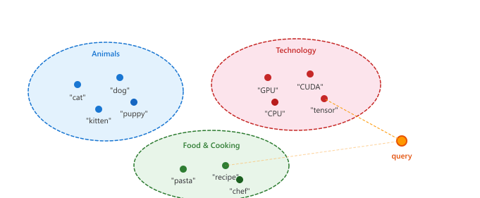
In high-dimensional spaces, distances between points tend to concentrate: the difference between the nearest and farthest neighbor shrinks relative to the overall distance. This phenomenon, known as the curse of dimensionality, means that exact nearest neighbor search becomes less meaningful as dimensionality grows. In practice, this is why approximate nearest neighbor (ANN) algorithms work so well for embeddings: the approximation error introduced by ANN is often smaller than the noise inherent in high-dimensional distance computations. Figure 31.2.3a shows how semantic clustering emerges in embedding space.
31.2.4 Fine-Tuning Embeddings for Domain Specificity
General-purpose embedding models may not capture domain-specific terminology or relationships well. For example, in a legal domain, "consideration" means something entirely different from its everyday usage. Fine-tuning an embedding model on domain-specific data can substantially improve retrieval quality.
# Fine-tuning a sentence transformer on domain-specific data
from sentence_transformers import (
    SentenceTransformer,
    SentenceTransformerTrainer,
    SentenceTransformerTrainingArguments,
    losses,
)
from datasets import Dataset
# Prepare training data: (anchor, positive) pairs
# Hard negatives are automatically mined from in-batch examples
train_data = Dataset.from_dict({
    "anchor": [
    "What is consideration in contract law?",
    "Define the doctrine of estoppel",
    "What constitutes a breach of fiduciary duty?",
    ],
    "positive": [
    "Consideration is something of value exchanged between parties to a contract.",
    "Estoppel prevents a party from asserting a claim inconsistent with prior conduct.",
    "A fiduciary breach occurs when a fiduciary acts against the beneficiary interest.",
    ],
})
# Load base model
model = SentenceTransformer("sentence-transformers/all-MiniLM-L6-v2")
# Configure training
loss = losses.MultipleNegativesRankingLoss(model)
args = SentenceTransformerTrainingArguments(
    output_dir="./legal-embedding-model",
    num_train_epochs=3,
    per_device_train_batch_size=32,
    learning_rate=2e-5,
    warmup_ratio=0.1,
    fp16=True,
)
trainer = SentenceTransformerTrainer(
    model=model,
    args=args,
    train_dataset=train_data,
    loss=loss,
)
trainer.train()
model.save_pretrained("./legal-embedding-model")Effective embedding fine-tuning typically requires at least 1,000 to 10,000 query-passage pairs from your domain. Start with a strong general-purpose base model (such as bge-large-en-v1.5 or GTE-large) rather than training from scratch. Use a small learning rate (1e-5 to 3e-5) and monitor validation retrieval metrics (recall@10, MRR@10) to detect overfitting early. If you have limited labeled data, consider using LLM-generated synthetic queries to augment your training set.
31.2.5 Practical Considerations
Theory and fine-tuning aside, three production gotchas catch nearly every team shipping their first embedding pipeline. The first is instruction prefixes, where forgetting "query: " or "passage: " can silently halve recall. The second is the asymmetry between query-time and document-time processing, and the third is batched re-embedding when models are versioned. We address them in that order.
Query and Document Prefixes
Many modern embedding models (E5, BGE, GTE) use instruction prefixes to distinguish
between different input types. For example, the E5 model family expects queries to be prefixed with
"query: " and documents with "passage: ". Forgetting these prefixes can
significantly degrade retrieval performance. Always check the model documentation for required
formatting conventions.
Sequence Length and Truncation
Every embedding model has a maximum sequence length, beyond which input is truncated. Older models like all-MiniLM-L6-v2 support only 256 tokens, while newer models such as nomic-embed-text-v1.5 and GTE-Qwen2 handle 8,192 or even 32,768 tokens. When your documents exceed the model's limit, you must chunk them before embedding, which is covered in detail in Section 31.6.
Batch Size and Throughput
Embedding throughput scales linearly with batch size up to the GPU memory limit. For production workloads, encode documents in large batches (256 to 1024) to maximize GPU utilization. For real-time query encoding, latency is more important than throughput, so smaller batch sizes (1 to 16) are typical. Consider using ONNX Runtime or TensorRT for optimized inference if you are serving embeddings at scale.
Always L2-normalize your embedding vectors before inserting them into a vector database. This converts cosine similarity to simple dot product, which is faster to compute and supported natively by all vector databases.
Who: A senior ML engineer at a 200-person legal technology startup
Situation: The company needed to build a semantic search system over 4 million legal documents (contracts, briefs, case law) to help paralegals find relevant precedents.
Problem: General-purpose embedding models (e.g., all-MiniLM-L6-v2) scored well on MTEB benchmarks but returned poor results on domain-specific queries like "force majeure clause triggered by pandemic."
Dilemma: A larger model (e5-large-v2, 1024 dimensions) offered better retrieval quality but required 4x the storage and doubled query latency. Fine-tuning a smaller model required 5,000 labeled query/passage pairs, which would take two weeks to annotate.
Decision: The team chose to fine-tune e5-base-v2 (768 dimensions) using 3,000 pairs curated from existing attorney search logs, supplemented with 2,000 synthetic pairs generated by GPT-4.
How: They used sentence-transformers with MultipleNegativesRankingLoss, mining hard negatives from BM25 results. Training took 6 hours on a single A100 GPU.
Result: Recall@10 improved from 62% to 84% on their internal legal benchmark, while keeping latency under 50ms per query. Storage stayed manageable at 12 GB for the full index.
Lesson: Domain-specific fine-tuning on a moderate-sized model often outperforms a larger general model, especially when you can mine training data from real user interactions.
Matryoshka and adaptive-dimension embeddings (Kusupati et al., NeurIPS 2022) allow a single model to produce embeddings at multiple dimensionalities, letting practitioners trade off between quality and storage/speed without retraining. Instruction-tuned embeddings (e.g., E5-Mistral, GritLM) embed the task description into the query, producing embeddings that are optimized for the specific retrieval, classification, or clustering task at hand.
Meanwhile, multilingual embedding models are closing the gap between English and low-resource languages through contrastive pretraining on parallel corpora. Research into embedding model distillation is producing smaller models (under 100M parameters) that match the quality of billion-parameter encoders on domain-specific benchmarks, a critical development for edge deployment.
Objective
Load multiple embedding models, encode a document collection, build a semantic search engine using cosine similarity, and benchmark the models against each other on retrieval quality.
What You'll Practice
- Loading and using sentence-transformers embedding models
- Computing cosine similarity between query and document embeddings
- Building a simple vector search index from scratch
- Evaluating retrieval quality with precision@k
Setup
The following cell installs the required packages and configures the environment for this lab.
Steps
Step 1: Load two embedding models
Load a small and a large embedding model to compare their behavior.
from sentence_transformers import SentenceTransformer
import numpy as np
model_small = SentenceTransformer("all-MiniLM-L6-v2") # 80MB, 384 dims
model_large = SentenceTransformer("all-mpnet-base-v2") # 420MB, 768 dims
print(f"Small: {model_small.get_sentence_embedding_dimension()} dims")
print(f"Large: {model_large.get_sentence_embedding_dimension()} dims")
# Quick test
test = "Machine learning is a subset of artificial intelligence."
print(f"Small shape: {model_small.encode(test).shape}")
print(f"Large shape: {model_large.encode(test).shape}")Hint
SentenceTransformer automatically downloads model weights on first use. If memory is limited, you can use just the small model for the lab.
Step 2: Build and encode a document collection
Create a diverse set of documents and encode them all into vectors.
documents = [
    "Python is a high-level programming language known for readability.",
    "Neural networks are computing systems inspired by biological brains.",
    "The Great Wall of China is over 13,000 miles long.",
    "Photosynthesis converts sunlight into chemical energy in plants.",
    "JavaScript is the most popular language for web development.",
    "Deep learning uses multiple layers of neural networks.",
    "The Amazon rainforest produces 20% of the world's oxygen.",
    "SQL is used for managing and querying relational databases.",
    "Climate change is causing rising sea levels worldwide.",
    "Transfer learning lets models trained on one task help with another.",
    "The human genome contains approximately 3 billion base pairs.",
    "Docker containers package applications with their dependencies.",
    "Coral reefs support 25% of all marine species.",
    "Gradient descent is the core optimization algorithm in deep learning.",
    "The International Space Station orbits Earth every 90 minutes.",
]
# TODO: Encode all documents with both models
embeddings_small = model_small.encode(documents)
embeddings_large = model_large.encode(documents)
print(f"Small embeddings: {embeddings_small.shape}")
print(f"Large embeddings: {embeddings_large.shape}")Hint
Passing the full list to model.encode(documents) is much faster than encoding one at a time because it batches the computation.
Step 3: Implement semantic search
Build a search function using cosine similarity.
import numpy as np
def semantic_search(query, model, doc_embeddings, documents, top_k=3):
    """Find the top-k most similar documents to the query."""
    # TODO: Encode the query, compute cosine similarity, return top-k
    query_emb = model.encode(query)
    norms = np.linalg.norm(doc_embeddings, axis=1) * np.linalg.norm(query_emb)
    scores = np.dot(doc_embeddings, query_emb) / norms
    top_idx = np.argsort(scores)[::-1][:top_k]
    return [(documents[i], scores[i], i) for i in top_idx]
# Test
queries = [
    "How do plants make food from sunlight?",
    "What programming language is best for web apps?",
    "Tell me about artificial intelligence techniques",
    "What are some environmental issues?",
    ]
for query in queries:
    print(f"\nQuery: {query}")
    for doc, score, _ in semantic_search(query, model_small, embeddings_small, documents):
        print(f" [{score:.3f}] {doc[:70]}...")
Hint
Cosine similarity: dot(a, b) / (norm(a) * norm(b)). Use np.argsort(scores)[::-1][:top_k] to get the indices of the highest-scoring documents.
Step 4: Benchmark the two models
Compare retrieval quality using queries with known relevant documents.
import pandas as pd
ground_truth = {
    "How do plants make food from sunlight?": [3],
    "What programming language is best for web apps?": [4],
    "Tell me about AI techniques": [1, 5, 9, 13],
    "What are environmental issues?": [8, 6, 12],
    }
def precision_at_k(retrieved_idx, relevant_idx, k=3):
    return len(set(retrieved_idx[:k]) & set(relevant_idx)) / k
results = []
for query, relevant in ground_truth.items():
    for name, mdl, embs in [("MiniLM", model_small, embeddings_small),
        ("MPNet", model_large, embeddings_large)]:
        hits = semantic_search(query, mdl, embs, documents, top_k=3)
        retrieved = [idx for _, _, idx in hits]
        p3 = precision_at_k(retrieved, relevant, k=3)
        results.append({"query": query[:40], "model": name, "P@3": p3})
        df = pd.DataFrame(results)
        print(df.to_string(index=False))
        print(f"\nAvg P@3 MiniLM: {df[df['model']=='MiniLM']['P@3'].mean():.3f}")
print(f"Avg P@3 MPNet: {df[df['model']=='MPNet']['P@3'].mean():.3f}")Hint
Precision@3 measures the fraction of top-3 results that are relevant. The larger model typically achieves equal or slightly better precision due to its richer representations.
Expected Output
- Semantic search returning sensible results (photosynthesis for plant queries, JavaScript for web dev)
- A comparison table showing P@3 scores for both models across all queries
- The larger model (MPNet) typically scoring the same or slightly better than MiniLM
Stretch Goals
- Add a third model (e.g., "BAAI/bge-small-en-v1.5") and extend the benchmark
- Measure encoding speed (documents per second) for each model and plot quality vs. speed
- Try Matryoshka truncation: use only the first 128 dimensions and re-run the benchmark
Complete Solution
from sentence_transformers import SentenceTransformer
import numpy as np, pandas as pd
model_small = SentenceTransformer("all-MiniLM-L6-v2")
model_large = SentenceTransformer("all-mpnet-base-v2")
documents = [
    "Python is a high-level programming language known for readability.",
    "Neural networks are computing systems inspired by biological brains.",
    "The Great Wall of China is over 13,000 miles long.",
    "Photosynthesis converts sunlight into chemical energy in plants.",
    "JavaScript is the most popular language for web development.",
    "Deep learning uses multiple layers of neural networks.",
    "The Amazon rainforest produces 20% of the world's oxygen.",
    "SQL is used for managing and querying relational databases.",
    "Climate change is causing rising sea levels worldwide.",
    "Transfer learning lets models trained on one task help with another.",
    "The human genome contains approximately 3 billion base pairs.",
    "Docker containers package applications with their dependencies.",
    "Coral reefs support 25% of all marine species.",
    "Gradient descent is the core optimization algorithm in deep learning.",
    "The International Space Station orbits Earth every 90 minutes.",
    ]
embs_s = model_small.encode(documents)
embs_l = model_large.encode(documents)
def search(query, model, embs, docs, k=3):
    qe = model.encode(query)
    scores = np.dot(embs, qe) / (np.linalg.norm(embs, axis=1) * np.linalg.norm(qe))
    idx = np.argsort(scores)[::-1][:k]
    return [(docs[i], scores[i], i) for i in idx]
for q in ["How do plants make food?", "Best language for web apps?",
    "AI techniques", "Environmental issues?"]:
    print(f"\n{q}")
    for d, s, _ in search(q, model_small, embs_s, documents):
        print(f" [{s:.3f}] {d[:70]}")
        gt = {"How do plants make food?": [3], "Best language for web apps?": [4],
            "AI techniques": [1,5,9,13], "Environmental issues?": [8,6,12]}
def p_at_k(ret, rel, k=3):
    return len(set(ret[:k]) & set(rel)) / k
rows = []
for q, rel in gt.items():
    for nm, m, e in [("MiniLM",model_small,embs_s),("MPNet",model_large,embs_l)]:
        ri = [i for _,_,i in search(q, m, e, documents)]
        rows.append({"query":q[:35],"model":nm,"P@3":p_at_k(ri, rel)})
        df = pd.DataFrame(rows)
        print("\n" + df.to_string(index=False))
        for m in ["MiniLM","MPNet"]:
print(f"Avg {m}: {df[df['model']==m]['P@3'].mean():.3f}")The whole search function collapses to a single cosine call plus an argsort. Useful in evaluation notebooks where you want a fast, dependency-light replacement before switching to FAISS at production scale.
Show code
from sklearn.metrics.pairwise import cosine_similarity
import numpy as np

def search(query, model, embs, docs, k=3):
    qe = model.encode([query])
    sims = cosine_similarity(qe, embs)[0]
    idx = np.argsort(sims)[::-1][:k]
return [(docs[i], sims[i], i) for i in idx]search() helper that ranks a precomputed embedding matrix against a query with sklearn.cosine_similarity and argsort, returning the top-k (document, score, index) triples.FAISS gives you sub-millisecond top-k over millions of vectors. Build an inner-product index over L2-normalized embeddings to recover the exact cosine ranking.
Show code
import faiss, numpy as np

embs = doc_embeddings.astype("float32")
faiss.normalize_L2(embs)
index = faiss.IndexFlatIP(embs.shape[1])
index.add(embs)

qe = model.encode([query]).astype("float32"); faiss.normalize_L2(qe)
scores, idx = index.search(qe, top_k)FAISS replaces the brute-force NumPy scan.- Bi-encoders enable scalable search by precomputing document embeddings, reducing query-time computation to a single dot product per candidate.
- Contrastive learning with in-batch negatives (MNRL/InfoNCE) is the standard training approach, and hard negative mining is critical for pushing embedding quality beyond baseline levels.
- Matryoshka embeddings provide flexible dimensionality from a single model, enabling storage/accuracy tradeoffs without retraining.
- ColBERT's late interaction preserves per-token information for better accuracy at the cost of higher storage requirements.
- Always evaluate on your data. MTEB scores provide a starting point, but domain-specific evaluation is essential for production model selection.
- L2-normalize your embeddings to simplify metric choices and enable the fastest similarity computation (dot product).
- Fine-tuning on 1K to 10K domain pairs can dramatically improve retrieval quality for specialized applications.
Show Answer
Show Answer
Show Answer
Show Answer
Show Answer
Exercises
Explain why a bi-encoder is preferred over a cross-encoder for large-scale retrieval, even though cross-encoders are more accurate. Under what conditions would you use a cross-encoder instead?
Show Answer
Bi-encoders encode query and documents independently, allowing precomputation. Cross-encoders require joint encoding of every query-document pair, which is $O(N)$ per query. Use cross-encoders for reranking a small candidate set (top 20 to 50) after bi-encoder retrieval.
In contrastive learning, what happens if all the negative samples in a batch are too easy (very different from the anchor)? How does hard negative mining address this?
Show Answer
Easy negatives provide almost no gradient signal because the model already distinguishes them. Hard negative mining selects negatives that are close to the anchor in embedding space, forcing the model to learn finer distinctions. Without it, the model plateaus quickly.
Explain how Matryoshka Representation Learning allows a single model to produce useful embeddings at multiple dimensionalities. Why is it better than simply training separate models at each dimension?
Show Answer
MRL trains the model so that truncating the embedding vector to any prefix still produces a useful representation. The information is hierarchically packed: the most important dimensions come first. Training separate models at each dimension would require N models and N times the compute.
A colleague stores embeddings in a vector database using dot product similarity but uses a model trained with cosine similarity loss. What problems might arise, and how would you fix them?
Show Answer
Dot product is not normalized, so vectors with larger magnitudes will dominate results regardless of semantic similarity. Either normalize embeddings before storing (making dot product equivalent to cosine), or switch the database to cosine similarity metric.
You have an embedding model trained on general web text, but your application involves legal contracts. Describe two strategies for adapting the model to the legal domain, and explain the tradeoffs between them.
Show Answer
(a) Contrastive fine-tuning on legal sentence pairs (higher quality, requires labeled pairs). (b) Continued pretraining on legal text with a masked language modeling objective (no labels needed, but less targeted). Fine-tuning is more effective when you have at least a few hundred labeled pairs.
Use sentence-transformers to embed 10 sentences from two distinct topics (e.g., cooking and programming). Compute pairwise cosine similarities and visualize the similarity matrix as a heatmap. Do within-topic similarities consistently exceed cross-topic similarities?
Take a model that supports Matryoshka embeddings (e.g., nomic-embed-text-v1.5). Embed 100 sentence pairs and measure retrieval accuracy (Recall@5) at dimensions 768, 384, 128, and 64. At what dimension does quality degrade noticeably?
Using an instruction-tuned model like E5, embed the same text with and without the query/passage prefix. Compare the resulting vectors using cosine similarity. How much does the prefix change the embedding?
Using the sentence-transformers training API, fine-tune a small embedding model on a domain-specific dataset (e.g., StackOverflow question pairs). Compare retrieval performance before and after fine-tuning on a held-out test set.
What Comes Next
In the next section, Section 31.3: Vector Index Data Structures & Algorithms, we explore vector index data structures and algorithms (HNSW, IVF, PQ) that enable fast similarity search at scale.