Multimodal Evaluation: Vision-Language, Audio, Video

"A picture is worth a thousand tokens, but only if your eval can tell which thousand."

Eval, Pixel-Pedantic AI Agent

43.5.1 The Modality Matrix: Input, Output, and Everything In Between

The first step in setting up multimodal evaluation is to enumerate which modality combinations your system handles. The combinations matter more than the modalities themselves: image-in/text-out (visual question answering) is a fundamentally different problem from text-in/image-out (image generation), and they need different metrics, different benchmarks, and different judge models.

A useful mental model is a two-axis grid. The input axis lists the modalities the model consumes: text, image, audio, video, structured data (tables, charts), and screenshot (a special case of image with strong layout priors). The output axis lists the modalities the model produces: text, image, audio, video, and structured output (function calls, JSON). The cells of the grid are the eval regimes you actually need.

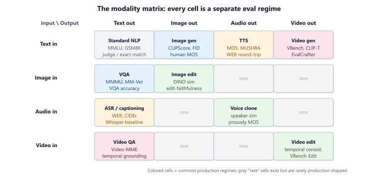
For a typical 2026 production agent, the relevant cells are usually four or five:

• Image-in, text-out (visual question answering, screenshot description, OCR-grounded reasoning): the largest body of benchmarks lives here. Metrics blend exact-match (for factual VQA), semantic similarity (for descriptive answers), and grounding accuracy (does the model point at the right region?).
• Audio-in, text-out (speech recognition, audio captioning, music tagging): dominated by word-error-rate (WER) and reference-based caption metrics. Reasonably mature.
• Text-in, image-out (image generation, image editing): dominated by CLIPScore for prompt fidelity, FID and KID for distributional realism, and human MOS-style scoring for aesthetic quality.
• Text-in, audio-out (text-to-speech, music generation): MOS, MUSHRA, and perceptual proxies like PESQ and ViSQOL. Highly subjective territory.
• Text-in, video-out (video generation): the youngest and least mature regime. VBench, EvalCrafter, and Veo/Sora-class evaluation harnesses are the current standards.

Two of the generation-quality metrics named above have a precise definition worth lifting out, because their range only makes sense once you see what they measure. FID (Frechet Inception Distance) embeds both the real and the generated images with a fixed encoder (the original proposal uses an Inception-v3 network; CLIP-based variants are now common), fits a Gaussian to each resulting feature cloud, and reports the Frechet (Wasserstein-2) distance between the two Gaussians:

$$\text{FID} = \lVert \mu_r - \mu_g \rVert^2 + \mathrm{Tr}\!\left(\Sigma_r + \Sigma_g - 2\,(\Sigma_r \Sigma_g)^{1/2}\right) .$$

Here $\mu_r, \Sigma_r$ are the mean and covariance of the real features and $\mu_g, \Sigma_g$ those of the generated features. The first term, $\lVert \mu_r - \mu_g \rVert^2$, is the squared gap between the two distribution centers (do the generated images sit, on average, where real images sit in feature space?), and the second term compares the covariance structure (do the generated images have the same spread and correlations across features?). FID is zero only when the two Gaussians coincide and grows as either the mean or the covariance diverges, so lower is better. KID (Kernel Inception Distance) measures the same distributional gap but as the squared maximum mean discrepancy (MMD) between the two feature sets under a polynomial kernel; unlike FID it is an unbiased estimator, so it stays reliable on the small sample sizes where FID's Gaussian fit is itself noisy.

One subtlety: in many 2026 production systems, the same model handles multiple modality combinations. GPT-4o, Gemini 2.5, and Claude Opus all consume images and audio while emitting text and (in some configurations) audio. The "single model, many combinations" pattern makes per-cell evaluation more important, not less: aggregating across cells obscures the failure modes that matter for each user-facing feature.

43.5.2 Vision-Language Evaluation

Vision-language evaluation has the deepest benchmark catalogue of any multimodal regime. The canonical benchmarks fall into four buckets, roughly ordered by difficulty:

• VQAv2 (Goyal et al., 2017): 1.1M open-ended questions about MS-COCO images, with balanced answer distributions. Easy by 2026 standards (frontier models score above 85%). Useful as a smoke test, not a discriminator.
• GQA (Hudson and Manning, 2019): compositional questions auto-generated from Visual Genome scene graphs. Tests counting, spatial relations, attribute comparison. Still meaningfully hard for small vision-language models.
• MMMU (Yue et al., 2024): 11,500 multi-discipline multimodal questions at college-exam level, spanning art, business, science, engineering. The reference benchmark for "does this model understand textbook-style figures?" Frontier models in 2025 score in the 60-70 range; humans score around 88.
• MM-Vet (Yu et al., 2024): 218 hard examples covering six integrated capabilities (recognition, OCR, knowledge, language generation, spatial awareness, math). Discriminative even among frontier models.

In production, you rarely run these benchmarks as written. Instead, you adapt the methodology: build a domain-specific eval set with the same question structure (multiple-choice for MMMU-style, open-ended with multi-reference scoring for VQA-style), and use the published scoring code to keep numbers comparable to the literature.

CLIPScore and its limits

CLIPScore (Hessel et al., 2021) is the workhorse metric for image-text alignment without a text reference. It computes the cosine similarity between a CLIP image embedding and a CLIP text embedding, then rescales to a 0-100 range. Its main virtue is that it does not require human-written captions: you can score generated text against the source image directly.

# Input: an image path and a caption string
# Output: CLIPScore in [0, 100] measuring image-caption alignment
import torch
from PIL import Image
from transformers import CLIPProcessor, CLIPModel

model = CLIPModel.from_pretrained("openai/clip-vit-large-patch14")
proc  = CLIPProcessor.from_pretrained("openai/clip-vit-large-patch14")

def clipscore(image_path: str, caption: str) -> float:
    image   = Image.open(image_path).convert("RGB")
    inputs  = proc(text=[caption], images=image, return_tensors="pt", padding=True)
    with torch.no_grad():
        out     = model(**inputs)
    img_emb = out.image_embeds / out.image_embeds.norm(dim=-1, keepdim=True)
    txt_emb = out.text_embeds  / out.text_embeds.norm(dim=-1, keepdim=True)
    cos     = (img_emb * txt_emb).sum(dim=-1).item()
    return max(0, 100 * 2.5 * cos)   # Hessel et al. recommended w=2.5

print(clipscore("cat.jpg", "a tabby cat sleeping on a sunlit windowsill"))

CLIPScore has well-documented failure modes. It is insensitive to fine-grained correctness ("a brown dog" and "a brown cat" can score similarly if both match the background), it can be gamed by stuffing the caption with rare visually grounded nouns, and it inherits any bias present in the CLIP training corpus (LAION-style web pairs). Treat CLIPScore as a fast, cheap first-pass filter; pair it with task-specific metrics (VQA accuracy for question answering, CIDEr or SPICE when references exist) before making a release decision.

Screenshot grounding for web and GUI agents

Browser-using agents (the WebArena family, OSWorld, AgentBench's web split) require a different kind of vision-language eval: visual element matching. The model is shown a screenshot, asked to click a specific element, and the eval checks whether the predicted bounding box overlaps the ground-truth element. The standard metrics are IoU (intersection-over-union) at thresholds 0.25, 0.5, 0.75, and center-point accuracy (did the click land inside the element?).

The hard part is that production GUI agents emit pixel coordinates, not bounding boxes; the eval has to map clicks back to DOM elements (in browser cases) or to OCR-extracted regions (in pure-screenshot cases). WebArena resolves this by running the model's clicks against a real headless browser and scoring task completion downstream, which is more faithful to the user experience but much slower and noisier than a static IoU eval.

43.5.3 Audio Generation Evaluation

Audio output evaluation is older than LLM evaluation by several decades, and the metric landscape reflects that history. The traditional speech-synthesis literature divides metrics into three tiers: subjective listening tests, perceptual quality proxies, and content-fidelity scores.

MOS (Mean Opinion Score) is the gold standard for subjective audio quality. Listeners rate samples on a 1-5 scale (1 = bad, 5 = excellent), and the system score is the mean over many ratings. ITU-T Recommendation P.808 defines a crowdsourced MOS protocol that has become the de facto industry standard. The fundamental limitation is cost: a stable MOS estimate requires hundreds of listeners per condition, and the variance between studies makes cross-paper comparison unreliable.

MUSHRA (MUlti-Stimulus test with Hidden Reference and Anchor), defined in ITU-R BS.1534, is the more rigorous cousin of MOS. Listeners rate multiple systems on the same screen, with a hidden reference (high anchor) and a deliberately degraded low anchor; the relative scoring controls for listener-level rating drift. MUSHRA is the standard for high-quality audio (music codecs, neural vocoders) where MOS rating ceilings get crowded.

PESQ (Perceptual Evaluation of Speech Quality) and ViSQOL (Virtual Speech Quality Objective Listener) are automatic proxies for MOS. They model human auditory perception with hand-crafted (PESQ) or learned (ViSQOL v3) features. Both correlate reasonably well with MOS on conventional codec degradations, but they were trained on bandwidth-limited telephony audio and tend to mis-score modern neural-vocoder artifacts (smooth, low-distortion audio that nevertheless sounds wrong to humans). Use them as cheap CI gates, not as release decisions.

Prompt-adherence for TTS is a separate axis: does the generated speech actually say the requested text? The simplest metric is to run an ASR model (Whisper-large works well) over the generated audio and compute WER against the original prompt. A good neural TTS system should score WER below 3%; if WER drifts upward, something is breaking before listeners notice. For prosody and emotion, the field is still without a strong automatic metric, and most teams fall back on listening tests for the prosodic dimensions.

Music generation evaluation introduces yet another set of metrics. The MusicGen and Stable Audio papers report Fréchet Audio Distance (FAD), the audio analog of FID for images. FAD measures the distance between feature-space distributions of generated and reference clips (typically using VGGish or CLAP audio embeddings). Lower is better; under 4.0 is considered competitive on the MusicCaps benchmark.

43.5.4 Video Generation Evaluation

Video generation is the newest and least mature of the modality regimes. Veo, Sora, Mochi, Kling, and the open-source models in their wake all rely on a handful of benchmarks that the field is still negotiating.

VBench (Huang et al., 2024) decomposes video quality into 16 dimensions: subject consistency, background consistency, temporal flickering, motion smoothness, dynamic degree, aesthetic quality, imaging quality, object class accuracy, multiple objects, human action recognition, color consistency, spatial relationships, scene consistency, appearance style, temporal style, and overall consistency. Each dimension has its own automatic scorer (a mix of CLIP-based, classifier-based, and optical-flow-based metrics). The total VBench score is a weighted average, but the per-dimension scores are what matter for diagnosis.

EvalCrafter (Liu et al., 2024) focuses on prompt-fidelity: does the generated video match the input text prompt? It scores along 17 axes including object recognition, action recognition, color matching, and motion description. It combines CLIP-T (CLIP text-image similarity, averaged across frames), action recognition scores from VideoCLIP, and text-conditioned video quality from a learned regressor.

Temporal-consistency metrics deserve their own attention. The simplest is per-frame CLIPScore between consecutive frames (high values mean the scene stays consistent), but this rewards static videos. The harder version is identity-preserving consistency: do the same characters and objects keep their identity over a 10-second clip? Subject-consistency benchmarks (VBench's "subject_consistency" score) use DINO-V2 feature similarity between detected subjects across frames as a proxy.

Motion smoothness is typically measured with optical-flow-based metrics: estimate dense flow with RAFT or GMFlow, then score the smoothness and physical plausibility of the resulting flow field. A model that produces sharp per-frame images but jagged motion will score well on per-frame quality and poorly on motion smoothness.

Prompt fidelity over frames

The standard text-to-video prompt-fidelity metric, CLIP-T over frames, samples N frames uniformly from the generated video, computes CLIPScore between the prompt and each frame, and averages. This is fast but coarse: it treats the prompt as a single attribute that must hold for every frame, when in practice prompts often describe actions (which only certain frames depict) or temporal events. EvalCrafter's action-recognition CLIP-T attempts to fix this by using action-grounded video encoders (VideoCLIP, X-CLIP) instead of frame-level CLIP, scoring against the action portion of the prompt rather than the static-scene portion.

43.5.5 Multimodal RAG Evaluation

The 3-layer cake from Section 35.1 (retrieval, generation, end-to-end) extends to multimodal RAG with one extra layer: cross-modal retrieval.

In a text-only RAG system, retrieval recall is a single number: of the K chunks fetched, how many were relevant? In a multimodal RAG system, retrieval has at least three sub-metrics:

• Text-to-image recall: given a text query, does the retriever return the right images? Standard recall@K against a labeled set.
• Image-to-text recall: given an image query (a screenshot, a photo), does the retriever return the right text passages? Standard recall@K, often run with CLIP or BLIP-2 as the cross-modal encoder.
• Table and chart extraction accuracy: for documents with embedded structured content, did the retriever's extractor convert tables and charts into queryable text (or structured) representations correctly? Metrics here are domain-specific: table-cell exact-match for financial documents, chart-element recall for scientific papers.

The second tier (generation) measures whether the model used the retrieved multimodal context. The faithfulness-style metrics from Section 35.1 generalize: did every claim in the answer have support in the retrieved image OR text OR table? The hard part is that "support in an image" is harder to verify than "support in a text passage": you typically need a vision-language judge to check whether a specific claim is visible in a specific region of an image.

The third tier (end-to-end) is the same as text-only RAG: did the user's task get done? For multimodal RAG (typical use case: ask a question about a PDF that contains both text and figures), end-to-end accuracy is usually measured against a held-out QA set with human-labeled answers.

43.5.6 Cross-Modal Grounding: Where Did the Model Actually Look?

The most subtle multimodal evaluation problem is grounding: when the model's text references an image region ("the red car in the top-left"), did the model actually attend to that region? This matters because models can produce text that looks grounded (correct region descriptions, plausible spatial language) while internally relying on language priors (red cars are usually mentioned in car-photo captions, regardless of which region they occupy).

Two methods dominate:

• Grad-CAM overlap: compute Grad-CAM saliency maps on the model's image encoder, restricted to the tokens of the grounding phrase. Compare the high-saliency regions to the ground-truth bounding box using IoU. High overlap = real grounding; low overlap = the model said the right thing for the wrong reason.
• Attention-mask IoU: for transformer-based vision-language models, extract the cross-attention weights from the text tokens of the grounding phrase to the image patches. Threshold and binarize the attention map, then compute IoU with the ground-truth box. Less interpretable than Grad-CAM but cheaper to compute.

Both methods are imperfect proxies for "where the model looked," but they catch the most egregious cases (the model says "the bird in the tree" while its attention is entirely on the ground). In safety-critical applications (medical imaging, autonomous driving simulation evaluation), grounding scores are increasingly part of the release gate alongside accuracy.

43.5.7 Hard Cases: Subjective Quality, Creative Output, Domain-Specific Multimodal

Three classes of multimodal evaluation remain genuinely hard in 2026, and budget-aware teams should plan around them rather than pretend the existing metrics solve them.

Audio aesthetic and emotional quality: a TTS system that achieves perfect WER and good PESQ can still sound robotic, monotone, or emotionally flat. There is no automatic metric that correlates well with "this voice sounds engaging." Production teams running large TTS deployments (Eleven Labs, OpenAI Voice, character.ai voice) all rely on weekly or biweekly listening panels to catch aesthetic regressions that automatic metrics miss. The same is true for music generation: FAD measures distributional realism but says nothing about whether a track is good.

Creative image and video output: when a user asks for "a surreal landscape," there is no single correct answer. CLIPScore measures prompt-fidelity, FID measures distributional realism, but neither captures originality, aesthetic intent, or artistic coherence. The standard solution is preference-based evaluation: have human raters compare pairs of outputs and compute Elo ratings (Chatbot Arena-style). Lmsys's Imagen Arena, ai.aest.io, and similar leaderboards have become the de facto external evaluation for generative image and video models.

Domain-specific multimodal: medical imaging, radiology reports, satellite imagery, scientific figures. Each domain has its own metrics that often combine multimodal accuracy with task-specific correctness. For radiology AI, the joint metric is often (a) classification accuracy on the imaging finding plus (b) clinical-correctness score on the generated text report, with both having to clear a threshold for the system to ship. The MIMIC-CXR-JPG and RadGraph benchmarks define the standard scoring code, but every hospital system ultimately runs its own internal evaluation against local data. Plan for domain-specific eval infrastructure as a multi-quarter effort, not a one-week build.

Exercises