"If your only evaluation metric is vibes, your only production guarantee is also vibes."
Eval, Vibe-Averse AI Agent
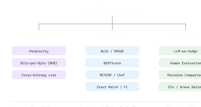
You cannot improve what you cannot measure, and measuring LLM quality is surprisingly hard. Unlike classification tasks where accuracy tells the whole story, LLM outputs are open-ended, subjective, and context-dependent. A single question can have many correct answers, each with different levels of helpfulness, style, and factual precision. This section builds your evaluation toolkit from low-level language modeling metrics (perplexity, bits-per-byte) through reference-based text metrics (BLEU, ROUGE, BERTScore), to modern approaches like LLM-as-Judge and structured human evaluation. It also covers the major benchmarks that the research community uses to track model capability over time. The decoding strategies from Section 4.2 (temperature, top-k, top-p) directly affect evaluation scores, so understanding their impact is essential for fair comparisons.
Prerequisites
This section assumes familiarity with LLM API patterns from Section 11.1 and prompt engineering from Section 12.1. Understanding basic ML evaluation concepts (precision, recall, F1) from Section 0.3 provides useful context for the evaluation metrics discussed here.
42.1.1 Intrinsic Language Modeling Metrics
When: any change to prompts, models, retrievers, or post-processors in a system with paying users. How: run a pinned 200-1000 example golden set on every PR; compute a small set of metrics (task accuracy, LLM-as-judge score, p95 cost, p95 latency); block the merge if any metric regresses by more than a pre-declared threshold (typically 2 percent for accuracy, 20 percent for cost). Watch for: noisy LLM-as-judge metrics (run with N=3 and average), golden-set rot (audit quarterly for stale or contested labels), and selection bias (your golden set should reflect production traffic, not your favorite test cases). Result: regressions caught at PR review instead of by users.
When evaluating at temperature > 0, set a fixed random seed and run at least three independent seeds. Report mean and standard deviation alongside your point estimate. A result sensitive to the seed choice is not a stable result. For greedy evaluation (T=0), one run is sufficient because outputs are deterministic per model and prompt. Many published LLM evals are single-seed temperature-1 runs, treat those numbers as provisional until replicated.
LLM judges exhibit a strong position bias: GPT-4 as a judge prefers the first response 58-65% of the time regardless of quality (Zheng et al., 2023, MT-Bench). An eval pipeline that always presents the same model first will report inflated win rates. The fix is symmetric swap: run each pair in BOTH orders and only count consistent verdicts.
# Input: judge LLM, question, candidate answers a and b
# Output: winner ('a wins', 'b wins', 'tie / unreliable') after running the judge on both orderings
def judge_with_swap(judge, question, a, b):
    v1 = judge(question, a, b)      # a first
    v2 = judge(question, b, a)      # b first
    if v1 == "first" and v2 == "second":  return "a wins"
    if v1 == "second" and v2 == "first":  return "b wins"
    return "tie / unreliable"   # judge disagreed with itself
The tie rate is itself an informative metric: high tie rates indicate the judge is too weak to distinguish the candidates. Length bias (longer responses score higher) requires a separate length-controlled eval to detect.
Team B shipped a customer-classification feature with 95% accuracy on their internal eval set. Within two weeks, real users were complaining about miscategorized tickets at much higher rates than the eval suggested. The team thought the model regressed. Investigation found that the eval set was built from resolved tickets, tickets the company's human agents had already triaged and that, by virtue of being resolved, were the easier cases. The production traffic contained much more ambiguous, multi-issue, and edge-case tickets that the eval set never saw. Fix: stratified sampling of live traffic (including unresolved tickets) into the eval set. Lesson: if your eval set is constructed by selecting on the dependent variable, your reported accuracy is biased upward by an unknown amount.
Every metric in this chapter is a proxy for what you actually care about. Perplexity is a proxy for language quality; BLEU is a proxy for translation fidelity; LLM-as-Judge is a proxy for human preference; benchmark accuracy is a proxy for real-world capability. Goodhart's Law, "when a measure becomes a target, it ceases to be a good measure", is the dominant failure mode in LLM evaluation, and it shows up as benchmark saturation (Chapter 42.2), reward hacking (Chapter 20), citation hallucination in RAG (Chapter 23.9), and the metric-mirage debate around emergent abilities (Chapter 43). Treat every metric you encounter as a hypothesis about the proxy's faithfulness, not as a definition of quality. See the Conceptual Map for the full thesis.
Intrinsic metrics measure how well a model captures the statistical properties of language itself. These metrics are computed directly from the model's probability distributions over tokens, without requiring any downstream task. They are most useful for comparing base (pretrained) models and for monitoring training progress.
BLEU score was invented in 2002 for machine translation and is still the most cited evaluation metric in NLP. It essentially counts matching n-grams, which means a random word salad that happens to contain the right phrases can score surprisingly well.
Perplexity
Perplexity measures how "surprised" a model is by a sequence of text. Formally, it is the exponentiated average negative log-likelihood per token. A model that assigns high probability to the correct next token at every position will have low perplexity. Lower perplexity means the model is a better predictor of natural language.
For a sequence of N tokens, perplexity is defined as:
The exp-of-log sleight in the formula hides a simple picture. Imagine the model is forced to bet on the next token by spinning a roulette wheel. Perplexity is the number of equally-likely slots that wheel would need to deliver the same average surprise the model actually feels on real text. PPL = 5 means "on average, the model has narrowed the next token to about five plausible choices"; PPL = 30 means "the next token feels roughly one of thirty equally-plausible options"; PPL near the vocabulary size means the wheel is the whole vocabulary (a uniform-random baseline) and the model has learned nothing.
So if a base model hits PPL 12 on WikiText and a stronger model hits PPL 8, the better model has shrunk the roulette from twelve slots to eight at every step; a concrete picture of "compresses the world better" you can hold in your hand without remembering the negative-log-likelihood definition. The catch (one the formula does not advertise) is that the size of each slot depends on the tokenizer: a 50K-vocab model and a 100K-vocab model are spinning different physical wheels, so the slot counts are not directly comparable. That mismatch is what bits-per-byte, below, exists to fix.
Perplexity depends heavily on the tokenizer. A model that uses byte-pair encoding (Chapter 1) with a 50K vocabulary will have a different perplexity from one using a 100K vocabulary, even if both models are equally capable. This makes direct perplexity comparisons across model families unreliable.
Bits-per-Byte (BPB)
Bits-per-byte normalizes the language modeling loss by the number of UTF-8 bytes rather than tokens, making it comparable across tokenizers and vocabularies. BPB measures how many bits the model needs, on average, to encode each byte of the original text. In plain terms, a lower BPB means the model compresses text more efficiently, which reflects better language understanding. This is the preferred metric when comparing models with different tokenization schemes.
# implement compute_perplexity_and_bpb
import torch
from transformers import AutoModelForCausalLM, AutoTokenizer
def compute_perplexity_and_bpb(model_name: str, text: str):
    """Compute perplexity and bits-per-byte for a text sample."""
    tokenizer = AutoTokenizer.from_pretrained(model_name)
    model = AutoModelForCausalLM.from_pretrained(
        model_name, torch_dtype=torch.float16, device_map="auto"
        )
    encodings = tokenizer(text, return_tensors="pt")
    input_ids = encodings.input_ids.to(model.device)
    with torch.no_grad():
        outputs = model(input_ids, labels=input_ids)
        neg_log_likelihood = outputs.loss # average NLL per token
        num_tokens = input_ids.size(1)
        perplexity = torch.exp(neg_log_likelihood).item()
        # Bits-per-byte: convert nats to bits, normalize by bytes
        total_nll_bits = neg_log_likelihood.item() * num_tokens / torch.log(torch.tensor(2.0))
        num_bytes = len(text.encode("utf-8"))
        bpb = total_nll_bits / num_bytes
        return {
            "perplexity": round(perplexity, 2),
            "bits_per_byte": round(bpb.item(), 4),
            "num_tokens": num_tokens,
            "num_bytes": num_bytes
            }
        # Example usage
        text = "The transformer architecture revolutionized natural language processing."
        result = compute_perplexity_and_bpb("gpt2", text)
print(result)exp(NLL) where NLL is the average per-token negative log-likelihood, while BPB normalizes by byte count instead of token count, making it tokenizer-agnostic and the right metric for cross-tokenizer comparison.Perplexity and BPB only measure how well a model predicts text, not how useful or safe its generations are. A model with excellent perplexity may still produce hallucination, refuse safe requests, or generate harmful content. These metrics are necessary but far from sufficient for evaluating instruction-tuned or chat models. presents this taxonomy.
42.1.2 Reference-Based Text Metrics
Reference-based metrics compare model output against one or more "gold standard" reference texts. They originated in machine translation and summarization, where human-written references provide a ground truth. These metrics are fast, deterministic, and cheap to compute, but they share a fundamental limitation: they assume the reference text captures the space of acceptable answers, which is rarely true for open-ended generation.
BLEU, ROUGE, and BERTScore
| Metric | What It Measures | Best For | Limitation |
|---|---|---|---|
| BLEU | N-gram precision (how many n-grams in the output appear in the reference) | Machine translation | Ignores recall; penalizes valid paraphrases |
| ROUGE-L | Longest common subsequence between output and reference | Summarization | Surface-level overlap; misses semantic equivalence |
| ROUGE-N | N-gram recall (how many reference n-grams appear in the output) | Summarization | Same surface-level limitations as ROUGE-L |
| BERTScore | Cosine similarity of contextualized token embeddings | Any text comparison | Computationally expensive; correlation varies by task |
| METEOR | Unigram matching with stemming, synonyms, and paraphrase support | Machine translation | Complex; still surface-level for LLM outputs |
Among these metrics, BLEU is the most established. Understanding its formula clarifies both its strengths (penalizing short or repetitive outputs) and its limitations (ignoring meaning entirely):
BLEU Score.
BLEU measures modified n-gram precision with a brevity penalty. For candidate c against reference r:
$$\text{BLEU} = \text{BP} \cdot \exp( \sum _{n=1..N} w_{n} \cdot \log(p_{n}) )$$where pn is the modified n-gram precision (clipped to reference counts), wn = 1/N are uniform weights (typically N=4), and the brevity penalty is:
$$\text{BP} = \min(1, \exp(1 - |r| / |c|))$$The brevity penalty penalizes candidates shorter than the reference, preventing trivially high precision from very short outputs.
Take candidate "the the the cat" (4 words) against reference "the cat sat on the mat" (6 words). BLEU clips each candidate word to its maximum count in the reference: "the" appears twice in the reference, so its three candidate occurrences are clipped to 2, and "cat" contributes 1. Clipped unigram precision is $p_1 = (2+1)/4 = 0.75$. Because the candidate (length $c=4$) is shorter than the reference (length $r=6$), the brevity penalty applies: $\mathrm{BP} = e^{1 - r/c} = e^{1 - 6/4} = e^{-0.5} \approx 0.61$. The BLEU-1 score is $\mathrm{BP}\times p_1 \approx 0.61 \times 0.75 \approx 0.46$, far below the naive 0.75, showing how clipping and the brevity penalty punish repetition and under-length output.
A complementary recall-oriented metric captures how much of the reference content appears in the candidate:
ROUGE-L (Longest Common Subsequence).
ROUGE-L uses the LCS between candidate c and reference r:
$$\begin{aligned}R_{\text{lcs}} &\text{amp};= \text{LCS}(r, c) / |r| ,\; P_{\text{lcs}} = \text{LCS}(r, c) / |c| \\ F_{\text{lcs}} &\text{amp};= (1 + \beta ^{2}) \cdot R_{\text{lcs}} \cdot P_{\text{lcs}} / ( \beta ^{2} \cdot P_{\text{lcs}} + R_{\text{lcs}})\end{aligned}$$where β controls the balance between precision and recall (typically β = 1.2, favoring recall).
Moving beyond surface-level matching, semantic similarity metrics use neural embeddings to capture meaning:
BERTScore.
BERTScore computes soft token matching using contextual embeddings. Given candidate tokens {ci} and reference tokens {rj} with their pretraining data embeddings:
$$\begin{aligned}P_{\text{BERT}} &\text{amp};= \frac{1}{|c|} \sum_{i} \max_{j} \cos(c_{i}, r_{j}) \\ R_{\text{BERT}} &\text{amp};= \frac{1}{|r|} \sum_{j} \max_{i} \cos(c_{i}, r_{j}) \\ F1_{\text{BERT}} &\text{amp};= \frac{2 \cdot P_{\text{BERT}} \cdot R_{\text{BERT}}}{P_{\text{BERT}} + R_{\text{BERT}}}\end{aligned}$$Each candidate token is matched to its most similar reference token (and vice versa) using cosine similarity of contextualized embeddings, capturing semantic equivalence that surface-level n-gram metrics miss.
METEOR scores a candidate by first building an explicit word alignment to the reference, matching not only exact tokens but also stems and synonyms (via WordNet) so paraphrases count. From the alignment it computes unigram precision and recall, then combines them as a recall-weighted harmonic mean, $F_{mean} = \frac{10 P R}{R + 9P}$. It then multiplies by a fragmentation penalty: the more the matched words are scattered into many non-contiguous chunks rather than long runs, the larger the penalty, which rewards correct word order. This alignment-plus-penalty design makes METEOR correlate with human judgment better than BLEU on segment-level machine translation, at higher compute cost.
# Implementation example
from rouge_score import rouge_scorer
from bert_score import score as bert_score
import evaluate
# Reference and candidate texts
reference = "The cat sat on the mat and watched the birds outside."
candidate = "A cat was sitting on a mat, observing birds through the window."
# ROUGE scores
scorer = rouge_scorer.RougeScorer(["rouge1", "rouge2", "rougeL"], use_stemmer=True)
rouge_results = scorer.score(reference, candidate)
for key, value in rouge_results.items():
    print(f"{key}: precision={value.precision:.3f}, recall={value.recall:.3f}, f1={value.fmeasure:.3f}")
    # BLEU score
    bleu = evaluate.load("bleu")
    bleu_result = bleu.compute(
        predictions=[candidate],
        references=[[reference]]
        )
    print(f"BLEU: {bleu_result['bleu']:.4f}")
    # BERTScore
    P, R, F1 = bert_score([candidate], [reference], lang="en", verbose=False)
print(f"BERTScore: precision={P[0]:.4f}, recall={R[0]:.4f}, f1={F1[0]:.4f}")Notice how BERTScore (0.94 F1) captures the semantic similarity between these paraphrases far better than BLEU (0.12) or ROUGE-2 (0.11). When outputs are valid paraphrases of references, embedding-based metrics like BERTScore provide much more meaningful signal. However, no single metric tells the full story. Use multiple metrics together and always validate against human judgment.
Why evaluation is harder for LLMs than classical ML. In classical ML, you measure a model's performance against a known ground truth: the cat is either correctly classified or it is not. LLM evaluation has no equivalent. A question like "Explain quantum computing" has thousands of valid answers that differ in depth, style, framing, and emphasis. Two responses can both be excellent yet share almost no words in common. This is why n-gram metrics like BLEU fail for open-ended generation: they reward surface overlap, not semantic quality. The field's migration from BLEU to BERTScore to LLM-as-Judge reflects a steady attempt to close this gap between what metrics measure and what users actually care about.
42.1.3 LLM-as-Judge
The LLM-as-Judge paradigm uses a strong language model (typically GPT-4, Claude, or a specialized judge model) to evaluate the outputs of other models. This approach has rapidly become the most popular evaluation method for instruction-tuned models because it can assess open-ended qualities like helpfulness, safety, and reasoning quality that reference-based metrics cannot capture.
When setting up LLM-as-Judge evaluation, always calibrate against human judgments first. Take 50 examples, have two humans rate them independently, then compare the judge model's ratings to both. If the judge agrees with humans less often than the humans agree with each other, your judge prompt needs revision before you scale up. This calibration step takes one afternoon and prevents weeks of misleading evaluation results.
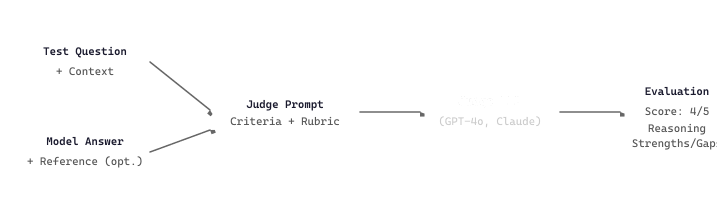
Judge Prompt Design
The quality of LLM-as-Judge evaluation depends entirely on the judge prompt. A well-designed prompt specifies clear evaluation criteria, provides a rubric with concrete examples at each score level, and asks the judge to produce a structured output (typically a score plus reasoning). The reasoning-before-score pattern (where the judge explains its rationale before assigning a numeric score) has been shown to produce more reliable evaluations.
# implement llm_judge_evaluate
from openai import OpenAI
import json
client = OpenAI()
def llm_judge_evaluate(question: str, answer: str, criteria: str) -> dict:
    """Use an LLM as a judge to evaluate answer quality."""
    judge_prompt = f"""You are an expert evaluator. Assess the following answer to a question.
    QUESTION: {question}
    ANSWER: {answer}
    EVALUATION CRITERIA: {criteria}
    RUBRIC:
    5 = Excellent: Fully addresses the question with accurate, comprehensive, well-organized content
    4 = Good: Addresses the question well with minor gaps or imprecisions
    3 = Adequate: Partially addresses the question but has notable gaps
    2 = Poor: Mostly fails to address the question or contains significant errors
    1 = Very Poor: Completely off-topic, factually wrong, or incoherent
    Provide your evaluation as JSON with these fields:
    - "reasoning": Your step-by-step analysis (2-3 sentences)
    - "score": Integer from 1 to 5
    - "strengths": List of strengths
    - "weaknesses": List of weaknesses"""
    response = client.chat.completions.create(
        model="gpt-4o",
        messages=[{"role": "user", "content": judge_prompt}],
        response_format={"type": "json_object"},
        temperature=0.0
    )
    return json.loads(response.choices[0].message.content)
# Example evaluation
result = llm_judge_evaluate(
    question="What causes seasons on Earth?",
    answer="Seasons happen because Earth's axis is tilted at 23.5 degrees relative to its orbital plane. This means different hemispheres receive more direct sunlight at different times of year.",
    criteria="Factual accuracy, completeness, and clarity"
)
print(json.dumps(result, indent=2))reasoning, score, strengths, and weaknesses fields, which lets downstream tooling aggregate rubric-level patterns rather than only a single number.Take the question "What causes seasons on Earth?" and the candidate answer "Seasons happen because Earth's axis is tilted at 23.5 degrees relative to its orbital plane. This means different hemispheres receive more direct sunlight at different times of year." Feeding this to the judge in Code Fragment 42.1.3a (with criteria "factual accuracy, completeness, and clarity") returns the JSON object
{
  "reasoning": "Correctly identifies axial tilt (23.5 deg) as the cause and explains the hemispheric sunlight mechanism clearly. Omits the role of orbital position and does not mention equinoxes or solstices.",
  "score": 4,
  "strengths": ["Correct identification of axial tilt", "Specific 23.5 degree figure", "Clear mechanism"],
  "weaknesses": ["No mention of orbital position", "Missing equinox / solstice details"]
}
The 4 on the rubric translates to "good with minor gaps", and the structured weaknesses list is what downstream tooling aggregates into a per-rubric heatmap. Re-running the same prompt at temperature 0 gives the same score; running it at temperature 0.7 across $N = 3$ seeds yields scores $\{4, 4, 5\}$ with mean $4.33$ and standard deviation $0.47$. The point estimate to report is the mean across seeds, and a one-step movement on the rubric is well within the per-judge noise, so a 0.5-point gap between two systems is not by itself meaningful evidence of a difference.
Reliability of an LLM-as-Judge pipeline is measured against a small held-out human-rated set. Given paired judge scores $(j_1, \ldots, j_n)$ and human scores $(h_1, \ldots, h_n)$, the Spearman rank correlation
captures how well the judge orders the candidates the same way humans do, even when the two scales differ in scale or offset. A Spearman correlation above 0.7 is the typical bar for treating an LLM-as-Judge metric as a credible proxy at scale, with the calibration set re-audited every quarter or whenever the judge model is upgraded (a judge swap from GPT-4o to GPT-5 can shift the score distribution by 0.3 to 0.5 points even when the rank order is preserved).
The same rubric runs against Claude with a near-identical interface; the swap is one line and useful for cross-checking judge biases (a GPT judge that scores its own outputs higher will not necessarily do so for Claude outputs).
Show code
import anthropic, json

client = anthropic.Anthropic()

def claude_judge(question: str, answer: str, criteria: str) -> dict:
    """One-shot LLM-as-Judge call against Claude, returns the same JSON shape as Code 42.1.3a."""
    rubric = (
        "5=Excellent, 4=Good, 3=Adequate, 2=Poor, 1=Very Poor.\n"
        "Return JSON with fields: reasoning, score, strengths, weaknesses."
    )
    msg = client.messages.create(
        model="claude-3-5-sonnet-latest",
        max_tokens=512,
        temperature=0.0,
        messages=[{"role": "user", "content": (
            f"QUESTION: {question}\nANSWER: {answer}\n"
            f"CRITERIA: {criteria}\nRUBRIC: {rubric}"
        )}],
    )
    return json.loads(msg.content[0].text)
Code Fragment 42.1.3c: The same Likert-rubric judge against Claude via the Anthropic SDK. Running both this and Code 42.1.3a on the same candidates and averaging is a cheap defense against self-preference bias.
The same result in 6 lines with DeepEval:
Show code
from deepeval.metrics import AnswerRelevancyMetric, FaithfulnessMetric
from deepeval.test_case import LLMTestCase
test_case = LLMTestCase(
    input="What causes seasons on Earth?",
    actual_output="Seasons happen because Earth's axis is tilted...",
    retrieval_context=["Earth's axis is tilted 23.5 degrees..."]
)
relevancy = AnswerRelevancyMetric(threshold=0.7)
relevancy.measure(test_case)
print(f"Score: {relevancy.score}, Reason: {relevancy.reason}")AnswerRelevancyMetric(threshold=0.7) wraps the rubric and JSON parsing internally, and measure(test_case) populates both a numeric score and a natural-language reason for debugging when a test fails CI.Common LLM-as-Judge Biases
LLM judges are powerful but carry systematic biases that evaluators must account for. Understanding these biases is essential for interpreting judge results correctly. Figure 42.1.2a shows the LLM-as-Judge evaluation pipeline.
- Position bias: Judges tend to prefer the first option in pairwise comparisons. Mitigation: randomize order and average scores across both orderings.
- Verbosity bias: Judges often favor longer, more detailed answers even when the extra content adds no value. Mitigation: include "conciseness is a virtue" in the rubric.
- Self-preference bias: Models tend to rate their own outputs higher than outputs from other models. Mitigation: use a judge model different from the models being evaluated.
- Authority bias: Confident, well-formatted answers receive higher scores even when factually wrong. Mitigation: explicitly instruct the judge to verify factual claims.
Position bias can be quantified with a position-balanced score. Let $s(A, B)$ be the probability that the judge picks A when A is shown first, and $s(B, A)$ the probability when B is shown first. The unbiased preference is
If a judge has no position bias, both terms are equal and $\hat{p}$ is just the raw win rate; if it has a strong "first answer wins" prior, the two terms diverge, and the average correctly de-biases the estimate.
# Position-balanced LLM-as-Judge for pairwise model comparison.
# Calls the judge twice per pair (A-then-B and B-then-A) and averages.
# This is the standard MT-Bench protocol; without the swap, position bias
# alone can inflate a model's apparent win rate by 5-15 percentage points.
import random
from openai import OpenAI

client = OpenAI()
RUBRIC = "You are an expert judge. Decide which answer is better. " \
         "Output exactly one of: 'A' or 'B'. Be concise. Avoid favoring " \
         "longer answers; conciseness is a virtue."

def judge_one_order(question, ans_first, ans_second, model="gpt-4o-mini"):
    prompt = (
        f"{RUBRIC}\n\nQuestion: {question}\n\n"
        f"Answer A:\n{ans_first}\n\nAnswer B:\n{ans_second}\n\nVerdict:"
    )
    r = client.chat.completions.create(
        model=model, temperature=0,
        messages=[{"role": "user", "content": prompt}],
    )
    return r.choices[0].message.content.strip().upper().startswith("A")

def pairwise_winrate(question, ans_X, ans_Y, n_trials=3):
    """Position-balanced win-rate of X over Y."""
    wins = 0
    for _ in range(n_trials):
        # Trial 1: X shown first.
        if judge_one_order(question, ans_X, ans_Y):
            wins += 1
        # Trial 2: X shown second.  Y is "A", X is "B"; we negate.
        if not judge_one_order(question, ans_Y, ans_X):
            wins += 1
    return wins / (2 * n_trials)
Code Fragment 42.1.2b: Position-balanced pairwise LLM-as-Judge. Each comparison runs twice (A first, then B first), and the answers are averaged so that the judge's position prior cancels out. This is the protocol used by MT-Bench, Arena-Hard, and most reproducible LLM leaderboards.
Suppose model X beats model Y on 60% of single-direction comparisons when X is shown first, but only 45% when X is shown second. The raw "X-first" win-rate of 60% looks like X dominates, but the symmetric estimate is $\hat{p}(X \succ Y) = \tfrac{1}{2}(0.60) + \tfrac{1}{2}(1 - 0.45) = 0.575$: X is mildly better, not strongly. A team running 100 questions and seeing 60 X-wins without swapping would miscalibrate the leaderboard by ~5 percentage points; on a benchmark like MT-Bench that decides go/no-go releases, that is the difference between "ship" and "retrain". This is why every reputable LLM benchmark since 2024 enforces position swapping as part of the protocol.
Intuitively, LLM-as-Judge works because strong models have internalized enough of human preferences through RLHF that they can approximate the judgment of a human annotator. The main risk is that the judge model shares the same biases as the model being evaluated (both prefer verbose, formal answers) creating a feedback loop that rewards style over substance. This is why calibrating LLM judges against human judgments, as described in the arena methodology of evaluation metrics, remains essential for high-stakes evaluation.
42.1.4 Human Evaluation
Human evaluation remains the gold standard for assessing LLM quality, especially for subjective dimensions like helpfulness, creativity, and conversational naturalness. However, human evaluation is expensive, slow, and introduces its own variability. The key challenge is designing evaluation protocols that are reliable (different annotators agree) and valid (they measure what you care about).
Evaluation Protocol Design
Effective human evaluation protocols share several characteristics. First, they define clear, specific criteria with concrete examples at each rating level. Second, they include calibration rounds where annotators evaluate the same examples and discuss disagreements before the main annotation begins. Third, they compute inter-annotator agreement metrics (like Cohen's kappa or Krippendorff's alpha) to verify that the task is well-defined enough for consistent human judgment.
Cohen's kappa corrects raw agreement for the agreement expected by chance: $\kappa = \dfrac{p_o - p_e}{1 - p_e}$, where $p_o$ is the observed proportion of items the two raters agree on and $p_e$ is the proportion expected if each rater labeled independently at their own base rates. Subtracting $p_e$ removes credit for lucky agreements (two raters who both answer "yes" 90% of the time start from a high $p_e$), and dividing by $1 - p_e$ rescales so that $\kappa = 1$ is perfect agreement and $\kappa = 0$ is chance level.
# implement compute_inter_annotator_agreement
import numpy as np
from sklearn.metrics import cohen_kappa_score
def compute_inter_annotator_agreement(annotations: dict) -> dict:
    """Compute pairwise Cohen's kappa between annotators.
    Args:
    annotations: dict mapping annotator_id to list of scores
    """
    annotator_ids = list(annotations.keys())
    kappas = {}
    for i in range(len(annotator_ids)):
        for j in range(i + 1, len(annotator_ids)):
            a1, a2 = annotator_ids[i], annotator_ids[j]
            kappa = cohen_kappa_score(
                annotations[a1], annotations[a2], weights="quadratic"
                )
            kappas[f"{a1}_vs_{a2}"] = round(kappa, 3)
            avg_kappa = np.mean(list(kappas.values()))
            return {"pairwise_kappas": kappas, "mean_kappa": round(avg_kappa, 3)}
            # Three annotators rating 10 examples on a 1-5 scale
            annotations = {
                "annotator_A": [4, 3, 5, 2, 4, 3, 5, 4, 3, 4],
                "annotator_B": [4, 3, 4, 2, 5, 3, 5, 3, 3, 4],
                "annotator_C": [5, 3, 5, 3, 4, 2, 4, 4, 3, 5],
                }
            agreement = compute_inter_annotator_agreement(annotations)
            print(f"Pairwise kappas: {agreement['pairwise_kappas']}")
            print(f"Mean kappa: {agreement['mean_kappa']}")
# Interpretation: >0.8 = excellent, 0.6-0.8 = good, 0.4-0.6 = moderateA mean kappa of 0.67 indicates "good" agreement, but the wide range (0.57 to 0.81) across annotator pairs suggests that annotator C may be interpreting the rubric differently. Before proceeding with annotation, run additional calibration rounds and review disagreement examples with all annotators to align their understanding of the scoring criteria.
42.1.5 Standard Benchmarks
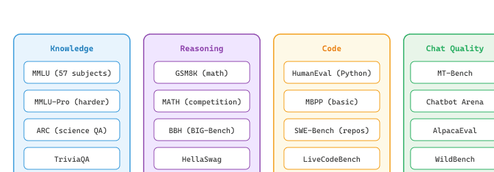
Benchmarks provide standardized test sets that enable comparison across models. The LLM community has developed dozens of benchmarks, each targeting different capabilities. Understanding what each benchmark measures (and what it does not measure) is essential for interpreting model comparison tables. Figure 42.1.3 maps the benchmark landscape by capability domain.
Benchmark Comparison
| Benchmark | Tasks | Metric | Format | Notes |
|---|---|---|---|---|
| MMLU | 57 subjects (STEM, humanities, social science) | Accuracy | Multiple choice | Most widely cited; saturation concern |
| HumanEval | 164 Python coding problems | pass@k | Code generation | Tests functional correctness via unit tests |
| MT-Bench | 80 multi-turn questions across 8 categories | LLM-as-Judge (1-10) | Open-ended | Tests multi-turn instruction following |
| Chatbot Arena | Crowdsourced pairwise comparisons | Elo rating (skill ranking derived from pairwise win/loss outcomes) | Side-by-side | Most ecologically valid; slow to update |
| GSM8K | 1,319 grade-school math word problems | Exact match | Free-form numeric | Nearly saturated by frontier models |
| SWE-Bench | Real GitHub issues requiring code fixes | % resolved | Repository-level code | Tests real-world software engineering; the 500-task SWE-bench Verified subset (OpenAI, 2024) removes mislabeled examples and is the production-quality variant |
| GPQA-Diamond | 198 PhD-level science questions (Rein et al., 2023) | Accuracy | Multiple choice (Google-proof) | Designed to resist web search; frontier reasoning models (o3, Gemini 2.5, Claude 3.7) reach 80-90% |
| Humanity's Last Exam (HLE) | 2,500 expert-curated questions across 100+ subjects (CAIS, 2025) | Accuracy | Mixed format | The MMLU successor: built specifically to remain hard for frontier models in 2025-26; top models score 20-30% |
| ARC-AGI-2 | Abstract reasoning puzzles (Chollet et al., March 2025) | Accuracy | Pattern completion | Released after o3 cracked ARC-AGI-1 in Dec 2024; frontier models still score under 10% as of mid-2025 |
| FrontierMath | Expert-level math problems (Epoch AI, 2024) | Exact answer | Free-form | Solutions take hours for trained mathematicians; frontier models score under 30% in 2025 |
Chatbot Arena ranks models using pairwise human comparisons rather than fixed benchmarks. The underlying Elo rating system, borrowed from chess, updates each model's score after every head-to-head comparison:
Elo Rating Update (Chatbot Arena).
After a comparison where model A (rating RA) plays against model B (rating RB), the expected win probability is:
$$E_{A} = 1 / (1 + 10^{(R_{B} - R_{A}) / 400})$$After observing actual outcome SA (1 for win, 0.5 for tie, 0 for loss), the rating updates as:
$$R_{A}^{\text{new}} = R_{A} + K \cdot (S_{A} - E_{A})$$where K is a sensitivity constant (typically 4 to 32). Chatbot Arena uses this to rank models from thousands of crowdsourced pairwise comparisons.
# implement run_mmlu_sample
import json
from datasets import load_dataset
def run_mmlu_sample(model_fn, num_samples: int = 20):
    """Evaluate a model on a sample of MMLU questions.
    Args:
    model_fn: callable that takes a prompt and returns A/B/C/D
    num_samples: number of questions to evaluate
    """
    dataset = load_dataset("cais/mmlu", "all", split="test")
    dataset = dataset.shuffle(seed=42).select(range(num_samples))
    correct = 0
    results_by_subject = {}
    for example in dataset:
        choices = example["choices"]
        prompt = f"""Question: {example['question']}
        A) {choices[0]}
        B) {choices[1]}
        C) {choices[2]}
        D) {choices[3]}
        Answer with just the letter (A, B, C, or D):"""
        prediction = model_fn(prompt).strip().upper()
        answer_map = {0: "A", 1: "B", 2: "C", 3: "D"}
        correct_letter = answer_map[example["answer"]]
        is_correct = prediction[0] == correct_letter if prediction else False
        subject = example["subject"]
        if subject not in results_by_subject:
            results_by_subject[subject] = {"correct": 0, "total": 0}
            results_by_subject[subject]["total"] += 1
            if is_correct:
                results_by_subject[subject]["correct"] += 1
                correct += 1
                accuracy = correct / num_samples
                return {
                    "overall_accuracy": round(accuracy, 3),
                    "num_correct": correct,
                    "num_total": num_samples,
                    "by_subject": results_by_subject
}shuffle(seed=42) makes the sample reproducible across runs, which is essential when comparing two checkpoints fairly.A growing concern with standard benchmarks is data contamination: the possibility that benchmark questions appeared in the model's training data. When a model has "seen" the test questions during training, its benchmark score overestimates true capability. Always check whether a model's technical report discusses contamination analysis, and consider using dynamic benchmarks (like LiveCodeBench or Chatbot Arena) that continuously add new questions.
The lm-eval-harness (pip install lm-eval) from EleutherAI is the standard framework for running reproducible LLM benchmarks. It supports 200+ tasks with consistent prompting, few-shot formatting, and scoring, and it is the engine behind the Open LLM Leaderboard.
Show code
# pip install lm-eval
# Command-line (most common):
# lm_eval --model hf \
# --model_args pretrained=meta-llama/Llama-3.1-8B-Instruct \
# --tasks mmlu,hellaswag,arc_challenge \
# --num_fewshot 5 \
# --batch_size auto \
# --output_path ./eval_results/
# Programmatic usage:
import lm_eval
results = lm_eval.simple_evaluate(
    model="hf",
    model_args="pretrained=meta-llama/Llama-3.1-8B-Instruct",
    tasks=["mmlu", "hellaswag"],
    num_fewshot=5,
    batch_size="auto",
    )
for task, metrics in results["results"].items():
    acc = metrics.get("acc,none", metrics.get("acc_norm,none", "N/A"))
print(f"{task}: {acc:.3f}")lm-eval-harness programmatic interface runs MMLU, HellaSwag, and ARC with consistent few-shot formatting and scoring. The batch_size="auto" argument tunes batch size to fit the available GPU memory, and simple_evaluate returns metrics under both acc (raw) and acc_norm (length-normalized) keys so you can pick the right one per task.42.1.6 Building an Evaluation Harness
In practice, you rarely evaluate with a single metric. A well-designed evaluation harness combines multiple metrics, runs them across a curated test set, and produces a structured report that tracks performance over time. The following example shows how to build a simple but extensible evaluation framework.
# Define EvalCase, EvalResult, EvalHarness; implement __init__, evaluate, summary
from dataclasses import dataclass, field
from typing import Callable
import json, time
@dataclass
class EvalCase:
    """A single evaluation test case."""
    question: str
    reference: str = ""
    metadata: dict = field(default_factory=dict)
@dataclass
class EvalResult:
    """Result of evaluating one test case."""
    case: EvalCase
    model_output: str
    scores: dict
    latency_ms: float
class EvalHarness:
    """Lightweight evaluation harness for LLM applications."""
    def __init__(self, model_fn: Callable, scorers: dict[str, Callable]):
        self.model_fn = model_fn # callable: prompt -> response
        self.scorers = scorers # dict of name -> scoring function
    def evaluate(self, cases: list[EvalCase]) -> list[EvalResult]:
        """Run all test cases through the model and score them."""
        results = []
        for case in cases:
            start = time.time()
            output = self.model_fn(case.question)
            latency = (time.time() - start) * 1000
            scores = {}
            for name, scorer in self.scorers.items():
                scores[name] = scorer(
                    question=case.question,
                    output=output,
                    reference=case.reference
                    )
                results.append(EvalResult(
                    case=case, model_output=output,
                    scores=scores, latency_ms=round(latency, 1)
                    ))
                return results
    def summary(self, results: list[EvalResult]) -> dict:
        """Aggregate results into a summary report."""
        import numpy as np
        metric_names = list(results[0].scores.keys())
        summary = {}
        for metric in metric_names:
            values = [r.scores[metric] for r in results]
            summary[metric] = {
                "mean": round(np.mean(values), 3),
                "std": round(np.std(values), 3),
                "min": round(min(values), 3),
                "max": round(max(values), 3),
                }
            summary["mean_latency_ms"] = round(
                np.mean([r.latency_ms for r in results]), 1
                )
return summaryEvalHarness that separates three concerns: test case management (EvalCase), model invocation (model_fn), and scoring (scorers dict). The summary method aggregates per-metric mean/std/min/max plus mean latency, producing the structured payload that downstream dashboards consume.The evaluation harness above builds scoring and test management from scratch for pedagogical clarity. In production, use DeepEval (install: pip install deepeval), which provides 14+ built-in metrics, pytest integration, and CI/CD support:
Show code
# Production evaluation using DeepEval
from deepeval import evaluate
from deepeval.test_case import LLMTestCase
from deepeval.metrics import AnswerRelevancyMetric, FaithfulnessMetric
test_case = LLMTestCase(
    input="What is Python?",
    actual_output=model_output,
    retrieval_context=["Python is a programming language..."]
)
evaluate([test_case], [AnswerRelevancyMetric(), FaithfulnessMetric()])evaluate function with built-in metrics (AnswerRelevancyMetric, FaithfulnessMetric). DeepEval handles latency tracking, parallel execution, and pytest integration internally, freeing you to focus on test case curation rather than plumbing.For CLI-driven evaluation with side-by-side comparisons, see promptfoo (install: npx promptfoo@latest init), which supports YAML-based test definitions and model comparison tables.
The best evaluation harnesses separate three concerns: (1) test case management (what to evaluate), (2) model invocation (how to get outputs), and (3) scoring (how to measure quality). This separation makes it easy to swap models, add new metrics, or reuse test cases across experiments. Start simple, then extend as your evaluation needs grow.
Who: ML engineering team at a SaaS company deploying an LLM-powered customer support assistant
Situation: The team had fine-tuned a model for customer support but lacked confidence in its readiness for production. Stakeholders asked for metrics, but the team was unsure which evaluation approach to trust.
Problem: BLEU scores against reference answers were misleading because valid responses could be phrased in many ways. A single benchmark score did not capture the multiple dimensions that mattered: helpfulness, factual accuracy, tone appropriateness, and safety.
Dilemma: Human evaluation was accurate but too slow and expensive for continuous testing. Automated metrics were fast but each had known biases (BERTScore favored verbose responses; LLM-as-Judge showed self-preference).
Decision: The team built a multi-layer evaluation harness combining automated metrics for fast screening, LLM-as-Judge with bias mitigation for quality assessment, and periodic human evaluation for calibration.
How: They created 500 test cases spanning 10 categories. Automated checks ran on every commit (response format, length, keyword presence). Weekly LLM-as-Judge evaluation used randomized answer ordering and multi-judge consensus to mitigate position and verbosity bias. Monthly human evaluation on 50 samples calibrated the automated scores.
Result: The harness caught a regression where a model update improved helpfulness scores but degraded safety responses, something no single metric would have detected. Time to evaluate went from 2 days (pure human) to 15 minutes (automated) with monthly calibration taking 4 hours.
Lesson: No single evaluation metric tells the full story; a layered approach combining fast automated checks, bias-mitigated LLM judges, and periodic human calibration provides both speed and reliability.
Automated metrics (BLEU, ROUGE, exact match) catch regressions quickly but miss nuance. Pair them with periodic human evaluation on a rotating sample. Even reviewing 20 outputs per week gives you a ground-truth signal that metrics alone cannot provide.
Open Questions in LLM Evaluation (2024-2026):
- Multi-dimensional evaluation: How can we build evaluation frameworks that simultaneously assess helpfulness, harmlessness, honesty, and instruction-following without collapsing these into a single score? Recent work on RLHF ensembles (2024-2025) shows promise but faces scaling challenges.
- Evaluation of reasoning chains: As reasoning models (o1, DeepSeek-R1) become standard, evaluating the quality of intermediate reasoning steps, not just final answers, remains an open problem. Process reward models offer one approach, but calibrating them is difficult.
- Cross-lingual evaluation gaps: Most benchmarks are English-centric. Multilingual evaluation suites like MEGA (2024) and Global MMLU are expanding coverage, but evaluation quality for low-resource languages remains poor.
Explore Further: Try implementing a multi-judge evaluation pipeline where three different LLMs score the same outputs and you measure inter-judge agreement, comparing it against human annotator agreement on the same examples.
- Perplexity measures prediction, not usefulness. Low perplexity is necessary but not sufficient for a good LLM. Instruction-tuned models may have higher perplexity than base models while being far more useful in practice.
- Reference-based metrics fail on open-ended tasks. BLEU and ROUGE penalize valid paraphrases. BERTScore captures semantics better but still cannot assess helpfulness, safety, or reasoning quality.
- LLM-as-Judge is powerful but biased. Account for position bias, verbosity bias, and self-preference bias through careful prompt design and evaluation protocol (order randomization, multi-judge consensus).
- Human evaluation requires rigorous protocol design. Define clear rubrics with concrete examples, run calibration rounds, and measure inter-annotator agreement before trusting human ratings.
- No single benchmark tells the full story. Evaluate across multiple dimensions (knowledge, reasoning, code, chat quality) and prefer dynamic benchmarks that resist contamination.
- Build evaluation harnesses early. Separating test cases, model invocation, and scoring into modular components makes your evaluation infrastructure reusable and extensible as your project evolves.
Show Answer
Show Answer
Show Answer
Show Answer
Show Answer
Exercises
Explain why perplexity scores cannot be directly compared between two models that use different tokenizers. What alternative metric avoids this problem?
Answer Sketch
Perplexity measures surprise per token, but different tokenizers split text into different numbers of tokens. A model with a larger vocabulary produces fewer tokens per sentence, so its per-token perplexity is computed over a different denominator. Bits-per-byte normalizes by the number of bytes in the original text, making it tokenizer-independent and enabling fair cross-model comparisons.
A model generates the sentence "The feline sat upon the mat" for the reference "The cat sat on the mat." Explain how BLEU and BERTScore would handle this case differently and which would give a higher score.
Answer Sketch
BLEU relies on exact n-gram overlap. "feline" and "upon" do not match "cat" and "on," so the unigram precision drops and higher-order n-gram matches are also lost. BERTScore computes cosine similarity between contextual embeddings, so "feline" and "cat" (as well as "upon" and "on") would have high embedding similarity. BERTScore would give a substantially higher score because it captures semantic equivalence rather than requiring lexical identity.
You use GPT-4 as a judge to evaluate outputs from GPT-4 and Claude. Identify at least three sources of bias in this setup and propose a mitigation for each.
Answer Sketch
(1) Self-enhancement bias: GPT-4 may prefer its own style. Mitigation: use a different judge model or multiple judges. (2) Position bias: the first response shown tends to be preferred. Mitigation: randomize presentation order or swap positions and average. (3) Verbosity bias: longer responses are often rated higher regardless of quality. Mitigation: include "prefer conciseness" in the rubric or normalize for length.
You are evaluating a customer support chatbot. Explain why MMLU would be a poor benchmark choice and propose three task-specific evaluation dimensions with example metrics for each.
Answer Sketch
MMLU tests broad factual knowledge through multiple-choice questions, which does not reflect customer support tasks (handling complaints, following policies, showing empathy). Better dimensions: (1) Accuracy: does the response correctly apply company policy? Metric: human-labeled correctness rate. (2) Helpfulness: does it resolve the user's issue? Metric: task completion rate. (3) Tone: is it empathetic and professional? Metric: LLM-as-judge rubric score on tone dimensions.
Write a Python function that takes a list of (generated_text, reference_text) pairs and computes ROUGE-L, BLEU, and a simple LLM-as-judge score (using an API call with a scoring rubric). Return a dictionary of aggregated metrics.
Answer Sketch
Use the rouge-score library for ROUGE-L and nltk.translate.bleu_score for BLEU. For LLM-as-judge, send each pair to an LLM with a rubric prompt asking for a 1-5 score, parse the integer from the response, and average across all pairs. Handle API errors gracefully and include the 95% confidence interval for each metric using bootstrap resampling.
What Comes Next
In the next section, Section 42.2: Experimental Design & Statistical Rigor, we cover experimental design and statistical rigor, ensuring that your evaluation results are reliable and actionable.