Part VIII's platforms split into evaluation services (which run the eval suites) and serving / observability services (which run the production traffic).
45.1.1 Evaluation platforms
- OpenAI Evals (OpenAI, 2023) is the open-source eval framework with a community-contributed registry of public evals. Its objective is to standardize how evals are written and run so any eval can be invoked against any OpenAI-compatible model with one command, which matters because eval reproducibility is otherwise terrible. The core concept is the Eval class with a sampler (the model under test) and a grader (the scoring function); evals are YAML-registered. Pick OpenAI Evals as the entry point for adding a benchmark to your CI; for advanced evals, Inspect AI is more powerful.
- Stanford HELM (Stanford CRFM, 2022) is the holistic eval platform that runs hundreds of metrics across dozens of models, publishing leaderboards on accuracy, robustness, fairness, bias, calibration, and efficiency. Its objective is to evaluate models on more than accuracy, which matters because a model that is 2 points more accurate but 20 points more biased is not a win. The core concept is "scenarios + metrics + models" as the cross product; reports are reproducible. Pick HELM for academic-rigorous multi-metric evaluation; for production CI, lighter tools are more practical.
- Inspect AI (UK AI Safety Institute, 2024) is AISI's eval framework, designed for safety and agentic evaluations, with native support for tool calling, sandboxed execution, and multi-turn dialogues. Its objective is to give safety researchers a framework that handles complex multi-step evals (where the model uses tools, makes multiple decisions, and reaches a final state), which matters because simple prompt-response evals miss agentic capabilities. The core concept is the Task abstraction with Solvers (what the model does) and Scorers (how to grade). Pick Inspect AI for agentic and safety evals; it has rapidly become the academic standard in 2025-2026.
- LangSmith (LangChain Inc., 2023) is the managed eval and tracing platform from the LangChain team, supporting both online tracing and offline eval datasets. Its objective is to make eval part of your normal LLM development cycle (write trace, capture, label, score), which matters when "vibes-based development" cannot scale past a few prompts. Pick LangSmith if you use LangChain; for standalone use, the eval features are still usable but the trace integration is tighter for LangChain-native apps.
- Braintrust (Braintrust Data, 2023) is an eval-first SaaS observability platform popular with prompt-engineering teams. Its objective is to make experiment-style eval workflows (try this prompt variant, compare against baseline, share results) the primary UX, which matters when your team iterates on prompts daily. The core concept is "experiments" (runs over an eval dataset) as first-class artifacts with diffing and trend tracking. Pick Braintrust for prompt-iteration-heavy workflows.
45.1.2 Serving platforms
- vLLM (UC Berkeley, 2023; now community-maintained) is the production-grade open-source inference server for LLMs. Its objective is to maximize tokens-per-second-per-GPU through PagedAttention and continuous batching, which matters when you serve more than 1 RPS to a real userbase. The core concept is treating KV cache as virtual memory with on-demand paging, eliminating fragmentation; think of it as a malloc for attention state. Pick vLLM when you need OpenAI-compatible serving with the best dollar-per-token economics; avoid when you need exotic decoding strategies vLLM has not shipped yet.
- Text Generation Inference (TGI) (Hugging Face, 2023) is the Hugging Face-stack production server that ships closely-integrated with the Transformers library. Its objective is to be the easiest path from a Hub model to a production endpoint, which matters when you already use HF models and want zero impedance mismatch. The core concept is the same continuous-batching pattern as vLLM with HF-first defaults. Pick TGI when ops simplicity inside the HF ecosystem outweighs vLLM's slightly higher throughput.
- SGLang (LMSYS, 2024) is vLLM's main competitor, focused on structured generation and complex prompt programs. Its objective is to optimize multi-turn, branching, and tool-calling workloads where vLLM's flat-prompt assumption breaks down, which matters in agentic loops. The core concept is RadixAttention: a prefix cache that shares KV state across requests with the same context prefix, plus a constraint-decoding DSL. Pick SGLang when prompts have large shared prefixes (multi-shot eval harnesses, agentic loops) or when you need fast JSON/grammar-constrained output.
- NVIDIA Triton (NVIDIA, 2018) is the framework-agnostic inference server that supports PyTorch, TensorFlow, ONNX, TensorRT, and arbitrary Python backends. Its objective is to host any model from any framework with a uniform gRPC and HTTP API, which matters when your production fleet runs heterogeneous models (LLMs, vision, traditional ML). Pick Triton for multi-framework production environments; for LLM-only serving, vLLM and TGI are simpler.
- TensorRT-LLM (NVIDIA, 2023) is NVIDIA's optimized inference runtime built on TensorRT specifically for transformer models. Its objective is to deliver the highest possible throughput on NVIDIA GPUs by compiling models to fused CUDA kernels at build time, which matters when you have a fixed model and need maximum tokens-per-second. The core concept is ahead-of-time engine compilation with quantization and kernel fusion. Pick TensorRT-LLM when single-model max-throughput matters; the build complexity makes it impractical for rapidly-iterating model lineups.
45.1.3 Observability platforms
- Arize (Arize AI, 2020) is the enterprise ML and LLM observability platform with strong drift detection and explainability. Its objective is to monitor production model behavior over time and surface degradations before users complain, which matters when your model serves millions of requests and silent quality drops are catastrophic. The core concept is per-feature distribution monitoring with drift alerts. Pick Arize for enterprise ML monitoring with established procurement; for self-serve, Phoenix is the open companion.
- Phoenix (Arize AI, 2023) is Arize's open-source companion for local tracing and eval, runnable on your laptop. Its objective is to be the free, hackable, OpenTelemetry-native tracing tool for LLM apps, which matters when you want to see traces during local development without paying for SaaS. Pick Phoenix for local dev and small-team observability; for enterprise scale, Arize is the upgrade path.
- Helicone (Helicone, 2023) is the proxy-based LLM observability platform: point your OpenAI client at Helicone's URL and every call is automatically logged. Its objective is zero-code-change observability, which matters when you want to add monitoring to existing code without refactoring. Pick Helicone for cost and latency visibility with minimal integration; for deeper trace inspection, Langfuse and LangSmith are stronger.
- Langfuse (Langfuse, 2023) is the open-source LangSmith competitor, runnable as SaaS or self-hosted via Docker. Its objective is to provide framework-agnostic LangSmith-shaped tracing without vendor lock-in, which matters when you want observability that survives a framework migration. Pick Langfuse when you need self-hosting or framework neutrality.
- Traceloop (Traceloop, 2023) is the OpenTelemetry-native LLM tracing platform, building on the OpenLLMetry standard. Its objective is to make LLM tracing first-class in your existing OpenTelemetry-based observability stack (Datadog, Honeycomb, Grafana), which matters when you already run OTel and do not want a second observability silo. Pick Traceloop when you already have OpenTelemetry infrastructure; for new deployments, Langfuse is more LLM-specific.
Inference Scaling and Load Balancing
Moving from a single-GPU inference setup to a production-grade serving cluster requires solving three problems: scaling (adding more GPU instances to handle growing traffic), load balancing (distributing requests intelligently across instances), and monitoring (knowing when to scale and diagnosing bottlenecks). This section covers horizontal and vertical scaling strategies, load balancer configurations, GPU utilization monitoring, tensor parallelism across multiple GPUs, throughput benchmarking, and cost optimization techniques.
1. Vertical vs. Horizontal Scaling
Two fundamental approaches handle more inference traffic. Vertical scaling means using a more powerful machine: more GPUs per node, faster GPUs, or more memory per GPU. This is often the right first step because it avoids distributed-systems complexity. A single node with 4 or 8 GPUs running tensor parallelism can serve surprisingly high throughput.
Horizontal scaling means running multiple independent inference instances behind a load balancer. Each instance holds a full copy of the model (or a tensor-parallel shard) and processes requests independently. This approach scales linearly: doubling the number of instances roughly doubles your throughput capacity.
Vertical scaling (tensor parallelism across GPUs within a node) reduces per-request latency because the model computation is split across GPUs. Horizontal scaling (multiple independent instances) increases total throughput without reducing per-request latency. In practice, you use both: tensor parallelism within each node for latency-sensitive models, and multiple nodes for capacity.
2. Multi-GPU Tensor Parallelism
For models too large for a single GPU, or when you need lower latency than a single GPU can provide, tensor parallelism splits the model across multiple GPUs within a single node. Each GPU holds a shard of the model's weight matrices and processes its portion of the computation in parallel. The GPUs synchronize via NVLink or PCIe after each attention and feed-forward layer.
All three serving frameworks support tensor parallelism through a simple configuration flag.
# vLLM: tensor parallelism across 4 GPUs
vllm serve meta-llama/Llama-3.1-70B-Instruct \
    --tensor-parallel-size 4 \
    --gpu-memory-utilization 0.90

# TGI: tensor parallelism across 4 GPUs
docker run --gpus all --shm-size 2g -p 8080:80 \
    -v /data:/data \
    ghcr.io/huggingface/text-generation-inference:latest \
    --model-id meta-llama/Llama-3.1-70B-Instruct \
    --num-shard 4

# SGLang: tensor parallelism across 4 GPUs
python -m sglang.launch_server \
    --model-path meta-llama/Llama-3.1-70B-Instruct \
--tp 4Tensor parallelism works best when the number of attention heads is evenly divisible by the tensor parallel size. For example, Llama-3.1 70B has 64 attention heads, so it shards cleanly across 1, 2, 4, or 8 GPUs. Using 3 or 5 GPUs would require padding and waste memory.
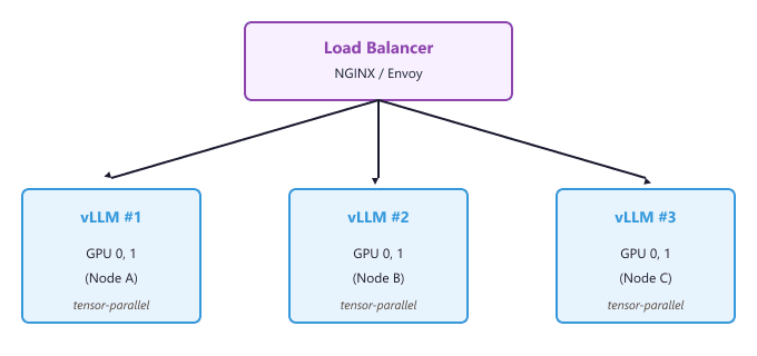
3. Load Balancing Strategies
A load balancer sits in front of your inference instances and routes incoming requests. The choice of routing algorithm significantly affects tail latency and throughput. The following configurations show NGINX and Envoy setups for LLM serving.
3.1 NGINX Configuration
The following NGINX configuration uses least-connections routing, which sends each new request to the instance with the fewest active connections. This works well for LLM serving because requests have variable processing times.
# /etc/nginx/nginx.conf
upstream vllm_cluster {
    least_conn;  # Route to instance with fewest active connections

    server node-a:8000 max_fails=3 fail_timeout=30s;
    server node-b:8000 max_fails=3 fail_timeout=30s;
    server node-c:8000 max_fails=3 fail_timeout=30s;
}

server {
    listen 80;

    # Increase timeouts for long-running generation requests
    proxy_read_timeout 300s;
    proxy_send_timeout 300s;

    location /v1/ {
        proxy_pass http://vllm_cluster;
        proxy_set_header Host $host;
        proxy_set_header X-Real-IP $remote_addr;

        # Enable streaming (SSE)
        proxy_buffering off;
        proxy_cache off;
        chunked_transfer_encoding on;
    }

    location /health {
        proxy_pass http://vllm_cluster;
    }
}3.2 Routing Algorithm Comparison
Different routing algorithms are suited to different workload patterns. The table below compares the most common options for LLM serving.
| Algorithm | Behavior | Best For |
|---|---|---|
| Round Robin | Cycles through instances sequentially | Uniform request sizes; simple deployments |
| Least Connections | Routes to the instance with fewest active requests | Variable output lengths; general-purpose LLM serving |
| Least Latency | Routes to the instance with the lowest recent response time | Heterogeneous GPU types in the same cluster |
| Session Affinity | Routes all requests from the same user to the same instance | Multi-turn chat with server-side KV cache persistence |
Avoid round-robin load balancing for LLM serving. Because requests have highly variable processing times (a 10-token response vs. a 2000-token response), round-robin frequently overloads one instance while others sit idle. Least-connections routing adapts to this variance automatically.
4. GPU Utilization Monitoring
Effective scaling requires visibility into GPU utilization, memory consumption, and queue depth. The
following Python script collects GPU metrics using the pynvml library and exposes them
in a format suitable for Prometheus or custom dashboards.
import pynvml
import time
import json

def collect_gpu_metrics():
    """Collect GPU metrics for all available devices."""
    pynvml.nvmlInit()
    device_count = pynvml.nvmlDeviceGetCount()
    metrics = []

    for i in range(device_count):
        handle = pynvml.nvmlDeviceGetHandleByIndex(i)
        util = pynvml.nvmlDeviceGetUtilizationRates(handle)
        mem_info = pynvml.nvmlDeviceGetMemoryInfo(handle)
        temp = pynvml.nvmlDeviceGetTemperature(handle, pynvml.NVML_TEMPERATURE_GPU)
        power = pynvml.nvmlDeviceGetPowerUsage(handle) / 1000  # milliwatts to watts

        metrics.append({
            "gpu_index": i,
            "gpu_utilization_pct": util.gpu,
            "memory_used_gb": round(mem_info.used / (1024 ** 3), 2),
            "memory_total_gb": round(mem_info.total / (1024 ** 3), 2),
            "memory_utilization_pct": round(mem_info.used / mem_info.total * 100, 1),
            "temperature_c": temp,
            "power_watts": round(power, 1),
        })

    pynvml.nvmlShutdown()
    return metrics

# Collect and display metrics every 5 seconds
while True:
    for m in collect_gpu_metrics():
        print(json.dumps(m))
    time.sleep(5)
For production deployments, integrate these metrics with Prometheus and Grafana. vLLM and TGI both
expose Prometheus-format metrics at their /metrics endpoints. The key metrics to
track for scaling decisions are listed below.
| Metric | Scaling Signal |
|---|---|
| Request queue depth | Scale up when queue consistently exceeds 2x your max batch size |
| GPU memory utilization | Above 95% indicates risk of OOM under burst load |
| Time to first token (TTFT) | Rising TTFT indicates the prefill phase is becoming a bottleneck |
| Tokens per second (throughput) | Flattening throughput despite increasing requests means capacity limit |
| GPU compute utilization | Below 60% with high queue depth suggests batching is suboptimal |
5. Benchmarking Throughput
Before deploying to production, benchmark your serving setup to understand its capacity limits. The following script sends concurrent requests to a vLLM or TGI server and measures throughput, latency percentiles, and time to first token.
import asyncio
import aiohttp
import time
import statistics

async def benchmark_serving(
    url: str,
    num_requests: int = 100,
    concurrency: int = 16,
    max_tokens: int = 128,
):
    """Benchmark an OpenAI-compatible serving endpoint."""
    semaphore = asyncio.Semaphore(concurrency)
    latencies = []
    first_token_times = []
    total_tokens = 0

    async def send_request(session, prompt):
        nonlocal total_tokens
        async with semaphore:
            start = time.perf_counter()
            first_token_time = None

            async with session.post(
                f"{url}/v1/completions",
                json={
                    "model": "default",
                    "prompt": prompt,
                    "max_tokens": max_tokens,
                    "temperature": 0.7,
                    "stream": True,
                },
            ) as resp:
                token_count = 0
                async for line in resp.content:
                    decoded = line.decode().strip()
                    if decoded.startswith("data:") and "[DONE]" not in decoded:
                        if first_token_time is None:
                            first_token_time = time.perf_counter() - start
                        token_count += 1

            elapsed = time.perf_counter() - start
            latencies.append(elapsed)
            if first_token_time:
                first_token_times.append(first_token_time)
            total_tokens += token_count

    prompts = [f"Write a short paragraph about topic number {i}." for i in range(num_requests)]

    start_time = time.perf_counter()
    async with aiohttp.ClientSession() as session:
        tasks = [send_request(session, p) for p in prompts]
        await asyncio.gather(*tasks)
    wall_time = time.perf_counter() - start_time

    print(f"Total requests:       {num_requests}")
    print(f"Concurrency:          {concurrency}")
    print(f"Wall clock time:      {wall_time:.2f}s")
    print(f"Throughput:           {total_tokens / wall_time:.1f} tokens/sec")
    print(f"Median latency:       {statistics.median(latencies):.3f}s")
    print(f"P95 latency:          {sorted(latencies)[int(0.95 * len(latencies))]:.3f}s")
    print(f"P99 latency:          {sorted(latencies)[int(0.99 * len(latencies))]:.3f}s")
    if first_token_times:
        print(f"Median TTFT:          {statistics.median(first_token_times):.3f}s")

# Run the benchmark
asyncio.run(benchmark_serving("http://localhost:8000", num_requests=200, concurrency=32))6. Cost Optimization Strategies
GPU inference is expensive, and optimizing costs requires attention at multiple levels. The following strategies can reduce serving costs by 40% to 70% without sacrificing quality or availability.
6.1 Right-Sizing Quantization
As covered in Section 9.2, quantization can cut GPU memory requirements by 4x. A 70B model quantized to 4 bits fits on a single A100-80GB instead of requiring two GPUs, halving your compute cost immediately. Benchmark your specific use case to verify that the quantized model meets your quality bar.
6.2 Autoscaling with Kubernetes
For workloads with variable traffic patterns, autoscaling inference pods based on GPU metrics avoids paying for idle capacity. The following Kubernetes configuration defines a Horizontal Pod Autoscaler that scales vLLM replicas based on GPU utilization.
# vllm-hpa.yaml
apiVersion: autoscaling/v2
kind: HorizontalPodAutoscaler
metadata:
  name: vllm-hpa
spec:
  scaleTargetRef:
    apiVersion: apps/v1
    kind: Deployment
    name: vllm-serving
  minReplicas: 1
  maxReplicas: 8
  metrics:
    - type: Pods
      pods:
        metric:
          name: gpu_utilization
        target:
          type: AverageValue
          averageValue: "75"    # Scale up when average GPU util exceeds 75%
  behavior:
    scaleDown:
      stabilizationWindowSeconds: 300  # Wait 5 min before scaling down
      policies:
        - type: Pods
          value: 1
          periodSeconds: 60
    scaleUp:
      stabilizationWindowSeconds: 30
      policies:
        - type: Pods
          value: 2
periodSeconds: 606.3 Spot and Preemptible Instances
Cloud providers offer GPU instances at 60% to 90% discounts through spot (AWS), preemptible (GCP), or low-priority (Azure) pricing. For inference workloads that can tolerate occasional interruptions, running a portion of your replicas on spot instances significantly reduces costs. Configure your load balancer to drain connections gracefully when a spot instance receives a termination notice.
A cost-effective production setup might use 2 on-demand vLLM replicas as a baseline (guaranteed availability) plus 4 spot instance replicas for burst capacity. The load balancer health checks automatically remove terminated spot instances, and the Kubernetes autoscaler replaces them when new spot capacity becomes available. This pattern reduces costs by roughly 50% compared to running all 6 replicas on-demand.
7. Production Checklist
Before deploying an LLM serving cluster to production, verify each item in the following checklist.
- Health checks: Load balancer probes the
/healthendpoint and removes unhealthy instances automatically - Graceful shutdown: Instances drain in-flight requests before terminating (set
terminationGracePeriodSecondsto at least 120) - Request timeouts: Proxy timeout set to at least 300 seconds for long completions; client-side timeout set slightly higher
- Rate limiting: Per-user or per-API-key rate limits prevent a single client from monopolizing the cluster
- Monitoring: Prometheus scraping GPU metrics, request latencies, and queue depth with Grafana dashboards and alerts
- Model versioning: Blue-green or canary deployment strategy for rolling out new model versions without downtime
- Logging: Structured request/response logging (excluding sensitive content) for debugging and audit
- Cost alerts: Budget alerts configured in your cloud provider to catch unexpected scaling events
Summary
Scaling LLM inference for production requires combining vertical scaling (tensor parallelism across GPUs) with horizontal scaling (multiple instances behind a load balancer). Least-connections routing handles the variable request durations inherent to autoregressive generation. Monitoring GPU utilization, queue depth, and time to first token provides the signals needed for autoscaling decisions. Cost optimization through quantization, spot instances, and right-sized autoscaling can reduce serving costs by 50% or more. With the techniques covered in this appendix, you have the tools to deploy, scale, and operate LLM inference in production across vLLM, TGI, and SGLang.
Production Data Pipelines and Serving at Scale
Production LLM systems require more than a trained model and a serving endpoint. They need data pipelines that continuously ingest, validate, and transform data; orchestration that coordinates training, evaluation, and deployment; monitoring that detects data drift and model degradation; and infrastructure that scales to handle unpredictable traffic. This section brings together the components from Sections O.1 through O.4 into end-to-end production architectures, covering pipeline orchestration with Airflow, CI/CD for ML, multi-model serving patterns, and observability for LLM systems.
End-to-End Pipeline Architecture
A production LLM pipeline typically consists of four stages: data ingestion (collecting raw data from APIs, databases, and event streams), data preparation (cleaning, filtering, and tokenizing into training-ready format), model training (fine-tuning or continued pretraining on prepared data), and deployment (packaging, validating, and serving the updated model). Each stage must be automated, idempotent, and observable.
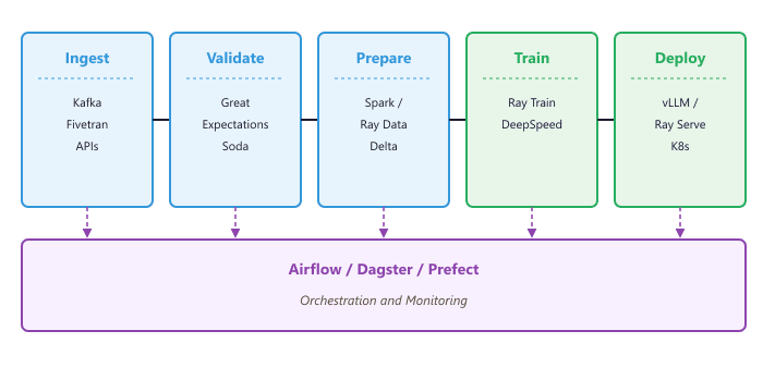
Pipeline Orchestration with Airflow
Apache Airflow is the most widely used orchestrator for ML pipelines. It represents workflows as directed acyclic graphs (DAGs) of tasks, with built-in support for scheduling, retries, alerting, and dependency management. For LLM pipelines, Airflow coordinates the steps that connect data preparation (using Spark on Databricks, as in Section 19.4 (Datasets & Benchmarks)) with distributed training (using Ray, as in Section 19.3 (Datasets & Benchmarks)) and deployment to an inference engine (as covered in Section 10.7 (vLLM Deep Dive)).
from airflow import DAG
from airflow.operators.python import PythonOperator
from airflow.providers.databricks.operators.databricks import (
    DatabricksRunNowOperator,
)
from airflow.providers.cncf.kubernetes.operators.pod import KubernetesPodOperator
from datetime import datetime, timedelta

default_args = {
    "owner": "ml-engineering",
    "retries": 2,
    "retry_delay": timedelta(minutes=10),
    "email_on_failure": True,
    "email": ["ml-team@company.com"],
}

with DAG(
    dag_id="llm_training_pipeline",
    default_args=default_args,
    schedule_interval="@weekly",
    start_date=datetime(2025, 1, 1),
    catchup=False,
    tags=["llm", "training"],
) as dag:

    # Step 1: Run data validation on the latest training data
    validate_data = DatabricksRunNowOperator(
        task_id="validate_training_data",
        databricks_conn_id="databricks_default",
        job_id=12345,  # Databricks job that runs Great Expectations
    )

    # Step 2: Prepare training data (tokenize, filter, split)
    prepare_data = DatabricksRunNowOperator(
        task_id="prepare_training_data",
        databricks_conn_id="databricks_default",
        job_id=12346,
    )

    # Step 3: Launch distributed training on Ray cluster
    train_model = KubernetesPodOperator(
        task_id="train_model",
        name="ray-training-job",
        image="company/ray-train:latest",
        cmds=["python", "train.py"],
        arguments=["--config", "configs/llama_sft.yaml"],
        namespace="ml-training",
        get_logs=True,
        startup_timeout_seconds=600,
    )

    # Step 4: Evaluate the trained model
    evaluate_model = KubernetesPodOperator(
        task_id="evaluate_model",
        name="model-evaluation",
        image="company/eval-harness:latest",
        cmds=["python", "evaluate.py"],
        namespace="ml-training",
    )

    # Define task dependencies
validate_data >> prepare_data >> train_model >> evaluate_modelUse Airflow's ShortCircuitOperator to skip downstream tasks when a validation step fails. For example, if data validation detects that fewer than 1,000 new examples have been added since the last training run, short-circuit the DAG to avoid wasting GPU hours on a training run that will produce negligible improvement.
Data Validation with Great Expectations
Data quality is the most common root cause of model degradation in production. Great Expectations is an open-source framework that lets you define expectations (assertions about your data) and run them automatically before each training run. For LLM training data, useful expectations include checking that instruction and response columns are non-null, that text lengths fall within expected ranges, and that quality scores meet a minimum threshold.
import great_expectations as gx

context = gx.get_context()

# Connect to a Delta Lake data source
datasource = context.data_sources.add_spark(name="delta_lake")
data_asset = datasource.add_dataframe_asset(name="instruction_pairs")

# Define expectations for training data quality
batch = data_asset.get_batch()
validator = context.get_validator(batch=batch)

# No null values in critical columns
validator.expect_column_values_to_not_be_null("instruction")
validator.expect_column_values_to_not_be_null("response")

# Text length within expected range (catch truncation or corruption)
validator.expect_column_value_lengths_to_be_between(
    "instruction", min_value=10, max_value=4096
)
validator.expect_column_value_lengths_to_be_between(
    "response", min_value=5, max_value=8192
)

# Quality score meets minimum threshold
validator.expect_column_values_to_be_between(
    "quality_score", min_value=0.6, max_value=1.0
)

# Run validation and check results
results = validator.validate()
if not results.success:
    failing = [r for r in results.results if not r.success]
    raise ValueError(
        f"Data validation failed: {len(failing)} expectations not met"
)CI/CD for ML: Automated Model Evaluation
Continuous integration for ML extends beyond code tests to include model evaluation. When a training pipeline produces a new model version, an automated evaluation step should run a standardized benchmark suite before the model is promoted to production. This prevents regressions where a newly trained model performs worse on specific tasks despite having a lower overall loss.
# .github/workflows/model-evaluation.yml
name: Model Evaluation Pipeline
on:
workflow_dispatch:
inputs:
model_version:
description: 'MLflow model version to evaluate'
required: true
model_name:
description: 'Registered model name'
default: 'ml_catalog.llm_models.llama_sft'
jobs:
evaluate:
runs-on: [self-hosted, gpu]
steps:
- uses: actions/checkout@v4
- name: Install dependencies
run: pip install mlflow vllm lm-eval
- name: Download model from MLflow
run: |
python scripts/download_model.py \
--model-name ${{ inputs.model_name }} \
--version ${{ inputs.model_version }} \
--output-dir ./model
- name: Run evaluation benchmarks
run: |
python -m lm_eval \
--model vllm \
--model_args pretrained=./model \
--tasks mmlu,hellaswag,truthfulqa \
--batch_size auto \
--output_path ./eval_results
- name: Check quality gates
run: |
python scripts/check_quality_gates.py \
--results ./eval_results \
--min-mmlu 0.65 \
--min-hellaswag 0.75 \
--max-regression 0.02
- name: Promote model if gates pass
if: success()
run: |
python scripts/promote_model.py \
--model-name ${{ inputs.model_name }} \
--version ${{ inputs.model_version }} \
--stage productionThe quality gate pattern is essential for production ML. Define explicit thresholds for each benchmark, and include a maximum regression check that compares the new model against the currently deployed version. A model can have excellent absolute scores but still be a regression on specific tasks that matter to your users. Always compare against the production baseline, not just a fixed threshold.
Multi-Model Serving Architecture
Production LLM applications rarely serve a single model. A typical deployment includes a primary generation model, an embedding model for retrieval, a reranker, and possibly a smaller classifier for intent routing. Managing these models requires an architecture that handles independent scaling, version management, and traffic routing for each model.
# Kubernetes deployment for multi-model serving with Ray Serve
# deploy_serving.py

from ray import serve
from ray.serve.config import AutoscalingConfig

@serve.deployment(
    autoscaling_config=AutoscalingConfig(
        min_replicas=2,
        max_replicas=10,
        target_ongoing_requests=5,
    ),
    ray_actor_options={"num_gpus": 1},
)
class GenerationModel:
    def __init__(self):
        from vllm import LLM
        self.llm = LLM(model="meta-llama/Llama-3.1-8B-Instruct")

@serve.deployment(
    autoscaling_config=AutoscalingConfig(
        min_replicas=1, max_replicas=4,
    ),
    ray_actor_options={"num_gpus": 0.5},
)
class EmbeddingModel:
    def __init__(self):
        from sentence_transformers import SentenceTransformer
        self.model = SentenceTransformer("BAAI/bge-large-en-v1.5")

    async def embed(self, texts):
        return self.model.encode(texts).tolist()

@serve.deployment(num_replicas=1)
class Router:
    def __init__(self, generator, embedder):
        self.generator = generator
        self.embedder = embedder

    async def __call__(self, request):
        data = await request.json()
        endpoint = data.get("endpoint", "generate")

        if endpoint == "embed":
            return await self.embedder.embed.remote(data["texts"])
        elif endpoint == "generate":
            return await self.generator.generate.remote(data["prompt"])

# Compose the application
generator = GenerationModel.bind()
embedder = EmbeddingModel.bind()
app = Router.bind(generator=generator, embedder=embedder)
serve.run(app, host="0.0.0.0", port=8000)Observability and Monitoring
LLM systems require monitoring beyond traditional application metrics. In addition to latency, throughput, and error rates, you need to track token usage (for cost management), output quality (for detecting model degradation), and data drift (for knowing when to retrain). Prometheus and Grafana provide the infrastructure layer, while specialized LLM observability tools like LangSmith, Langfuse, or Phoenix handle trace-level analysis of prompt chains and retrieval quality.
# Prometheus metrics for LLM serving
from prometheus_client import Counter, Histogram, Gauge, start_http_server

# Request-level metrics
REQUEST_COUNT = Counter(
    "llm_requests_total", "Total LLM requests",
    ["model", "endpoint", "status"]
)
REQUEST_LATENCY = Histogram(
    "llm_request_duration_seconds", "Request latency",
    ["model", "endpoint"],
    buckets=[0.1, 0.5, 1.0, 2.0, 5.0, 10.0, 30.0],
)
TOKENS_GENERATED = Counter(
    "llm_tokens_generated_total", "Total tokens generated",
    ["model"],
)
ACTIVE_REQUESTS = Gauge(
    "llm_active_requests", "Currently processing requests",
    ["model"],
)

# Start metrics endpoint
start_http_server(9090)

# Instrument your serving code
import time

async def serve_request(model_name, prompt):
    ACTIVE_REQUESTS.labels(model=model_name).inc()
    start = time.perf_counter()
    try:
        response = await generate(prompt)
        duration = time.perf_counter() - start

        REQUEST_COUNT.labels(
            model=model_name, endpoint="generate", status="success"
        ).inc()
        REQUEST_LATENCY.labels(
            model=model_name, endpoint="generate"
        ).observe(duration)
        TOKENS_GENERATED.labels(model=model_name).inc(
            response.usage.completion_tokens
        )
        return response
    except Exception as e:
        REQUEST_COUNT.labels(
            model=model_name, endpoint="generate", status="error"
        ).inc()
        raise
    finally:
ACTIVE_REQUESTS.labels(model=model_name).dec()Traditional ML monitoring tools are not sufficient for LLM systems. Input/output data drift detection requires embedding-based methods (not just statistical tests on numeric features), and output quality monitoring requires either automated evaluation with a judge model or structured human feedback loops. Budget for LLM-specific observability from the start; retrofitting it after launch is significantly harder.
Summary
Production LLM systems are distributed systems that require the same rigor as any critical infrastructure: automated pipelines, data validation, CI/CD with quality gates, multi-model serving, and comprehensive observability. Airflow or similar orchestrators coordinate the flow from data ingestion through training to deployment. Great Expectations catches data quality issues before they reach the model. CI/CD pipelines with benchmark evaluation prevent regressions. Multi-model serving architectures handle the reality that production LLM applications depend on several models working in concert. Finally, Prometheus metrics and LLM-specific observability tools provide the visibility needed to maintain reliability at scale. Together with the Databricks platform (Section 19.4 (Datasets & Benchmarks)), Delta Lake storage (Section 19.4 (Datasets & Benchmarks)), Ray compute (Section 19.3 (Datasets & Benchmarks)), and feature stores from the broader MLOps ecosystem, these components form a complete infrastructure stack for production LLM applications.
What's Next?
In the next section, Section 45.2: Libraries & Frameworks, we build on the material covered here.