I built a Transformer from scratch and it predicted "the the the the." Honestly, some meetings feel the same way.
Norm, Repetitively Decoded AI Agent
Prerequisites
This coding lab requires a solid understanding of the Transformer architecture from Section 4.1 and multi-head attention from Section 3.3. You will write PyTorch code, so the PyTorch tutorial in Section 0.3 (tensors, autograd, training loops) is essential preparation.
Reading about attention heads and layer normalization is one thing; implementing them is another. This hands-on lab translates the architecture from Section 4.1 into working PyTorch code, building a character-level language model step by step. By the end, you will have internalized how data flows through embeddings, multi-head attention, and feed-forward layers. This concrete understanding pays dividends when you fine-tune models in Chapter 14 or debug inference issues in production.
This section is a coding lab. By the end you will have a working character-level language model built on a decoder-only Transformer. Every line of code is explained. We encourage you to type the code yourself rather than copy-pasting; the act of typing builds muscle memory for these patterns.

1. What We Are Building
We will implement a decoder-only Transformer (the GPT architecture) that performs character-level language modeling. Given a sequence of characters, the model predicts the next character at every position. We choose character-level modeling because it eliminates the need for a tokenizer (Chapter 2), letting us focus entirely on the architecture.
Our model will have these hyperparameters:
| Hyperparameter | Value | Notes |
|---|---|---|
| d_model | 128 | Embedding and residual stream dimension |
| n_heads | 4 | Number of attention heads (d_k = 32) |
| n_layers | 4 | Number of Transformer blocks |
| d_ff | 512 | Feed-forward inner dimension (4 × d_model) |
| block_size | 128 | Maximum context length |
| vocab_size | ~65 | Unique characters in the dataset |
| dropout | 0.1 | Dropout rate |
This is a small model (~1.6M parameters) that trains in a few minutes on a single GPU (or even on CPU for a few epochs). The architecture is identical to GPT; only the scale differs.
Typing each line yourself forces you to read and understand every operation. You will notice patterns (the repeated LayerNorm, the residual connections, the projection matrices) that become invisible when you copy-paste. These patterns are the same ones you will encounter in every production Transformer codebase, from Hugging Face to vLLM.
2. The Complete Implementation
Below is the full model in a single file. We break it into logical pieces and explain each one. The complete code (all pieces assembled) is approximately 300 lines including comments.
2.1 Imports and Configuration
We begin by importing PyTorch and defining a configuration dataclass that holds all model hyperparameters.
"""
mini_transformer.py
A minimal decoder-only Transformer for character-level language modeling.
~300 lines of annotated PyTorch.
"""

import math
import torch
import torch.nn as nn
import torch.nn.functional as F
from dataclasses import dataclass

@dataclass
class TransformerConfig:
 """All hyperparameters in one place."""
 vocab_size: int = 65 # number of unique characters
 block_size: int = 128 # maximum context length
 n_layers: int = 4 # number of Transformer blocks
 n_heads: int = 4 # number of attention heads
 d_model: int = 128 # embedding / residual stream dimension
 d_ff: int = 512 # feed-forward inner dimension
 dropout: float = 0.1 # dropout probability
 bias: bool = False # use bias in Linear layers?
# Training loop for the mini-transformer: character-level batches,
# cross-entropy loss, AdamW optimizer with gradient clipping.

import time
from torch.utils.data import DataLoader

def train(config=None, text_path='input.txt', max_steps=5000,
 batch_size=64, learning_rate=3e-4, eval_interval=500):
 """Complete training procedure."""

 # ---- Setup ----
 device = 'cuda' if torch.cuda.is_available() else 'cpu'
 print(f"Using device: {device}")

 # Load text data
 with open(text_path, 'r', encoding='utf-8') as f:
 text = f.read()

 # Create dataset
 dataset = CharDataset(text, block_size=128)
 print(f"Vocabulary size: {dataset.vocab_size}")
 print(f"Dataset size: {len(dataset):,} examples")

 # Create config with correct vocab size
 if config is None:
 config = TransformerConfig(vocab_size=dataset.vocab_size)
 else:
 config.vocab_size = dataset.vocab_size

 # Create model
 model = MiniTransformer(config).to(device)
 n_params = sum(p.numel() for p in model.parameters())
 print(f"Model parameters: {n_params:,}")

 # Optimizer
 optimizer = torch.optim.AdamW(
 model.parameters(),
 lr=learning_rate,
 betas=(0.9, 0.95),
 weight_decay=0.1
 )

 # Data loader
 loader = DataLoader(dataset, batch_size=batch_size, shuffle=True,
 num_workers=0, pin_memory=True)
 data_iter = iter(loader)

 # ---- Training ----
 model.train()
 t0 = time.time()

 for step in range(max_steps):
 # Get batch (cycle through data)
 try:
 xb, yb = next(data_iter)
 except StopIteration:
 data_iter = iter(loader)
 xb, yb = next(data_iter)

 xb, yb = xb.to(device), yb.to(device)

 # Forward pass
 logits, loss = model(xb, yb)

 # Backward pass
 optimizer.zero_grad(set_to_none=True)
 loss.backward()

 # Gradient clipping (standard practice)
 torch.nn.utils.clip_grad_norm_(model.parameters(), max_norm=1.0)

 optimizer.step()

 # Logging
 if step % eval_interval == 0 or step == max_steps - 1:
 dt = time.time() - t0
 print(f"step {step:5d} | loss {loss.item():.4f} | "
 f"time {dt:.1f}s")

 # ---- Generation ----
 model.eval()
 prompt = "\n"
 context = torch.tensor(
 [dataset.encode(prompt)], dtype=torch.long, device=device
 )
 generated = model.generate(context, max_new_tokens=500, temperature=0.8)
 print("\n" + "=" * 50)
 print("Generated text:")
 print("=" * 50)
 print(dataset.decode(generated[0].tolist()))

 return model, dataset

if __name__ == '__main__':
 train()
We use a dataclass so that every hyperparameter is explicit, documented, and easy to
modify. Setting bias=False follows the LLaMA convention and marginally reduces
parameter count.
Code Fragment 4.2.2 below puts this into practice.
2.2 Causal Self-Attention
This module implements multi-head causal self-attention with a triangular mask that prevents positions from attending to future tokens.
# Causal self-attention with a triangular mask: each token can only
# attend to itself and earlier positions, enforcing left-to-right generation.

class CausalSelfAttention(nn.Module):
 """Multi-head causal (masked) self-attention."""

 def __init__(self, config: TransformerConfig):
 super().__init__()
 assert config.d_model % config.n_heads == 0

 # Key, Query, Value projections combined into one matrix
 self.qkv_proj = nn.Linear(config.d_model, 3 * config.d_model, bias=config.bias)
 # Output projection
 self.out_proj = nn.Linear(config.d_model, config.d_model, bias=config.bias)

 self.attn_dropout = nn.Dropout(config.dropout)
 self.resid_dropout = nn.Dropout(config.dropout)

 self.n_heads = config.n_heads
 self.d_model = config.d_model
 self.d_k = config.d_model // config.n_heads

 # Causal mask: lower-triangular boolean matrix
 # Register as buffer so it moves to GPU with the model
 mask = torch.tril(torch.ones(config.block_size, config.block_size))
 self.register_buffer("mask", mask.view(1, 1, config.block_size, config.block_size))

 def forward(self, x):
 B, T, C = x.shape # batch, sequence length, d_model

 # Compute Q, K, V in one matrix multiply, then split
 qkv = self.qkv_proj(x)
 q, k, v = qkv.split(self.d_model, dim=2)

 # Reshape for multi-head: (B, T, C) -> (B, n_heads, T, d_k)
 q = q.view(B, T, self.n_heads, self.d_k).transpose(1, 2)
 k = k.view(B, T, self.n_heads, self.d_k).transpose(1, 2)
 v = v.view(B, T, self.n_heads, self.d_k).transpose(1, 2)

 # Scaled dot-product attention
 # (B, n_heads, T, d_k) @ (B, n_heads, d_k, T) -> (B, n_heads, T, T)
 scores = (q @ k.transpose(-2, -1)) * (self.d_k ** -0.5)

 # Apply causal mask: positions beyond current token get -inf
 scores = scores.masked_fill(self.mask[:, :, :T, :T] == 0, float('-inf'))

 attn_weights = F.softmax(scores, dim=-1)
 attn_weights = self.attn_dropout(attn_weights)

 # Weighted sum of values
 # (B, n_heads, T, T) @ (B, n_heads, T, d_k) -> (B, n_heads, T, d_k)
 out = attn_weights @ v

 # Concatenate heads: (B, n_heads, T, d_k) -> (B, T, C)
 out = out.transpose(1, 2).contiguous().view(B, T, C)

 # Final linear projection + dropout
 return self.resid_dropout(self.out_proj(out))
Notice the line scores = (q @ k.transpose(-2, -1)) * (self.d_k ** -0.5). That
** -0.5 term (equivalent to dividing by √dk) is not cosmetic; it
prevents softmax from collapsing into a near-one-hot distribution.
Here is why. If the entries of Q and K are drawn roughly from a standard normal distribution (mean 0, variance 1), then each element of the dot product Q·K is the sum of dk products of independent unit-normal variables. By the properties of variance, the dot product has variance dk. For our config with dk = 32, this means raw scores have a standard deviation around 5 to 6. For a larger model with dk = 128, the standard deviation grows to about 11.
Feed values that large into softmax and the result becomes near-one-hot: almost all the attention weight concentrates on a single position, and the gradients of all other positions effectively vanish. The model stops learning. Dividing by √dk rescales the scores back to unit variance, keeping the softmax in a numerically healthy region where it produces diffuse distributions and carries gradients to all attended positions.
Concrete example: with dk = 128 and no scaling, a single score might be 14 while others cluster around 0. softmax(14, 0, 0, …) ≈ (0.9999, 0.00003, …). After dividing by √128 ≈ 11.3, the same score becomes ~1.2, and softmax produces a much more spread-out distribution where all positions can receive meaningful gradient signal. Section 4.3 explores how RoPE and other positional encodings interact with this scaling.
Our config uses n_heads=4, splitting dmodel=128 into four 32-dimensional
subspaces. Why not just do one big attention over all 128 dimensions?
Each head learns to attend to a different kind of relationship simultaneously. In a trained language model, different heads specialize in distinct patterns. Some heads focus on syntactic relationships: the subject attending to its verb, or a pronoun attending to its antecedent. Other heads capture positional patterns: attending to the immediately preceding token or to the first token in the sequence (a common "global anchor" behavior). Still others detect semantic similarity: tokens that occur in similar contexts across the corpus attracting one another.
If you used a single attention head over the full dmodel-dimensional space, the
attention weight at each position is a single scalar. Multiple heads produce
n_heads independent attention distributions over the sequence; the concatenation
of their weighted value outputs gives the model the ability to simultaneously retrieve
information along all these different relational axes. The output projection WO
then integrates these parallel "views" into a single updated representation.
Clark et al. (2019) visualized BERT's attention heads and found that individual heads develop
highly interpretable functions: one head predominantly attends to the
[SEP] separator token (global context anchor), another tracks direct objects of
verbs, and another follows coreference chains. These specializations emerge from training
alone; they are not explicitly programmed. See
Section 4.3 for more on attention head behavior.
We compute Q, K, and V with a single linear layer (qkv_proj) of size
d_model → 3 * d_model and then split the output into three equal parts.
This is mathematically identical to three separate linear layers but is more efficient because
it performs one large matrix multiply instead of three smaller ones. The GPU utilizes its
parallelism more effectively with larger matrices.
2.3 Feed-Forward Network
The position-wise feed-forward network applies two linear transformations with a nonlinearity in between.
# Position-wise FFN: expand to 4*d_model with ReLU, then project back.
# Applied independently at every token position in the sequence.

class FeedForward(nn.Module):
 """Position-wise feed-forward network with ReLU activation."""

 def __init__(self, config: TransformerConfig):
 super().__init__()
 self.fc1 = nn.Linear(config.d_model, config.d_ff, bias=config.bias)
 self.fc2 = nn.Linear(config.d_ff, config.d_model, bias=config.bias)
 self.dropout = nn.Dropout(config.dropout)

 # Forward pass: define computation graph
 def forward(self, x):
 x = F.relu(self.fc1(x))
 x = self.dropout(x)
 x = self.fc2(x)
 x = self.dropout(x)
 return x
This is the simplest version. For a more advanced variant, you can swap in SwiGLU. Code Fragment 4.2.4 below puts this into practice.
# SwiGLU FFN variant (LLaMA, PaLM): replace ReLU with a gated SiLU
# activation, using 2/3 of the hidden dimension for the gate projection.

class SwiGLUFeedForward(nn.Module):
 """SwiGLU feed-forward (used in LLaMA, PaLM)."""

 def __init__(self, config: TransformerConfig):
 super().__init__()
 # SwiGLU uses 3 weight matrices instead of 2
 # To keep param count comparable, the hidden dim is often 2/3 of d_ff
 hidden = int(2 * config.d_ff / 3)
 self.w1 = nn.Linear(config.d_model, hidden, bias=config.bias)
 self.w2 = nn.Linear(hidden, config.d_model, bias=config.bias)
 self.w3 = nn.Linear(config.d_model, hidden, bias=config.bias) # gate
 self.dropout = nn.Dropout(config.dropout)

 def forward(self, x):
 # SiLU(x * W1) * (x * W3) then project back
 return self.dropout(self.w2(F.silu(self.w1(x)) * self.w3(x)))
2.4 Transformer Block
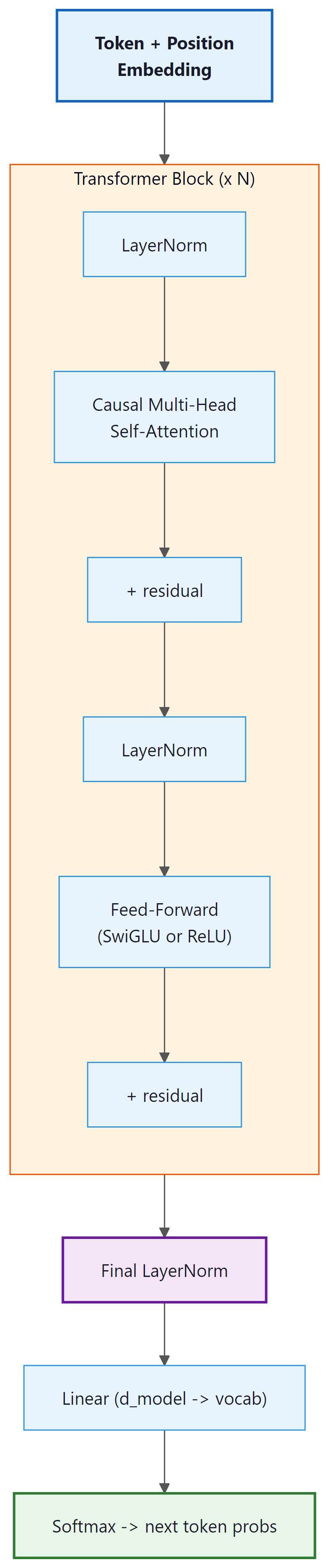
Each block combines causal self-attention and a feed-forward network with residual connections and layer normalization.
# Single transformer block: Pre-LN ordering with residual connections.
# Input flows through norm, attention, add residual, norm, FFN, add residual.

class TransformerBlock(nn.Module):
 """A single Transformer block with Pre-LN ordering."""

 def __init__(self, config: TransformerConfig):
 super().__init__()
 self.ln1 = nn.LayerNorm(config.d_model)
 self.attn = CausalSelfAttention(config)
 self.ln2 = nn.LayerNorm(config.d_model)
 self.ffn = FeedForward(config)

 # Forward pass: define computation graph
 def forward(self, x):
 # Pre-LN: normalize before each sub-layer
 x = x + self.attn(self.ln1(x)) # residual + attention
 x = x + self.ffn(self.ln2(x)) # residual + FFN
 return x
This is remarkably simple. Two lines of actual computation, each following the pattern:
x = x + SubLayer(LayerNorm(x)). The residual connection is the x + at the
beginning; the Pre-LN ordering means we normalize the input to each sub-layer, not the output.
The original "Attention Is All You Need" paper (Vaswani et al., 2017) placed LayerNorm
after the residual add: LayerNorm(x + SubLayer(x)). This is called
Post-LN. Our implementation uses Pre-LN: x + SubLayer(LayerNorm(x)).
That subtle reordering has a large practical effect.
With Post-LN, the gradients flowing back through the network must pass through the LayerNorm before reaching earlier layers. This creates large gradient variance that makes training unstable at large scale, requiring careful learning-rate warmup schedules. Pre-LN sends the raw residual gradient directly back to all earlier layers without passing through the norm, resulting in much more stable gradient flow. Virtually every modern LLM (GPT-2 onward, LLaMA, Mistral, Gemma) uses Pre-LN as a result.
There is also a simplified variant called RMSNorm (Zhang & Sennrich, 2019) that removes the mean-centering step of standard LayerNorm, keeping only the root-mean-square scaling. This reduces computation slightly with no measurable quality loss and is used in LLaMA, Mistral, and Qwen. For a full comparison of Post-LN, Pre-LN, and RMSNorm, including an architecture diagram, see Section 4.3: Pre-Norm vs. Post-Norm.
2.5 The Complete Model
The full model stacks an embedding layer, multiple Transformer blocks, and a final linear head for next-token prediction.
# Full decoder-only transformer: stack N blocks, add token + position
# embeddings, project to vocabulary logits, and implement autoregressive generate().

class MiniTransformer(nn.Module):
 """Decoder-only Transformer for character-level language modeling."""

 def __init__(self, config: TransformerConfig):
 super().__init__()
 self.config = config

 # Token and position embeddings
 self.token_emb = nn.Embedding(config.vocab_size, config.d_model)
 self.pos_emb = nn.Embedding(config.block_size, config.d_model)
 self.drop = nn.Dropout(config.dropout)

 # Stack of Transformer blocks
 self.blocks = nn.ModuleList([
 TransformerBlock(config) for _ in range(config.n_layers)
 ])

 # Final layer norm (needed with Pre-LN)
 self.ln_final = nn.LayerNorm(config.d_model)

 # Output head: project from d_model to vocab_size
 self.lm_head = nn.Linear(config.d_model, config.vocab_size, bias=False)

 # Weight tying: share embedding and output weights
 self.token_emb.weight = self.lm_head.weight

 # Initialize weights
 self.apply(self._init_weights)
 # Scale residual projections
 for block in self.blocks:
 nn.init.normal_(
 block.attn.out_proj.weight,
 mean=0.0,
 std=0.02 / math.sqrt(2 * config.n_layers)
 )
 nn.init.normal_(
 block.ffn.fc2.weight,
 mean=0.0,
 std=0.02 / math.sqrt(2 * config.n_layers)
 )

 def _init_weights(self, module):
 if isinstance(module, nn.Linear):
 nn.init.normal_(module.weight, mean=0.0, std=0.02)
 if module.bias is not None:
 nn.init.zeros_(module.bias)
 elif isinstance(module, nn.Embedding):
 nn.init.normal_(module.weight, mean=0.0, std=0.02)
 elif isinstance(module, nn.LayerNorm):
 nn.init.ones_(module.weight)
 nn.init.zeros_(module.bias)

 def forward(self, idx, targets=None):
 """
 Args:
 idx: (B, T) tensor of token indices
 targets: (B, T) tensor of target token indices (optional)
 Returns:
 logits: (B, T, vocab_size)
 loss: scalar cross-entropy loss (only if targets provided)
 """
 B, T = idx.shape
 assert T <= self.config.block_size, \
 f"Sequence length {T} exceeds block_size {self.config.block_size}"

 # Token embeddings + positional embeddings
 positions = torch.arange(0, T, device=idx.device) # (T,)
 x = self.token_emb(idx) + self.pos_emb(positions) # (B, T, d_model)
 x = self.drop(x)

 # Pass through all Transformer blocks
 for block in self.blocks:
 x = block(x)

 # Final normalization
 x = self.ln_final(x)

 # Project to vocabulary
 logits = self.lm_head(x) # (B, T, vocab_size)

 # Compute loss if targets are provided
 loss = None
 if targets is not None:
 loss = F.cross_entropy(
 logits.view(-1, logits.size(-1)),
 targets.view(-1)
 )

 return logits, loss

 @torch.no_grad()
 def generate(self, idx, max_new_tokens, temperature=1.0, top_k=None):
 """
 Auto-regressive generation.
 Args:
 idx: (B, T) conditioning sequence
 max_new_tokens: number of tokens to generate
 temperature: softmax temperature (lower = more deterministic)
 top_k: if set, only sample from top-k most likely tokens
 """
 for _ in range(max_new_tokens):
 # Crop context to block_size if needed
 idx_cond = idx[:, -self.config.block_size:]

 # Forward pass
 logits, _ = self(idx_cond)

 # Take logits at the last position and apply temperature
 logits = logits[:, -1, :] / temperature

 # Optional top-k filtering
 if top_k is not None:
 v, _ = torch.topk(logits, min(top_k, logits.size(-1)))
 logits[logits < v[:, [-1]]] = float('-inf')

 # Sample from the distribution
 probs = F.softmax(logits, dim=-1)
 next_token = torch.multinomial(probs, num_samples=1)

 # Append to sequence
 idx = torch.cat([idx, next_token], dim=1)

 return idx
The implementation above builds a complete decoder-only Transformer from scratch for pedagogical clarity. In production, use HuggingFace Transformers (install: pip install transformers), which provides pre-trained models and a standardized API:
# Production equivalent: load a pre-trained causal LM
from transformers import AutoModelForCausalLM, AutoTokenizer

model = AutoModelForCausalLM.from_pretrained("gpt2")
tokenizer = AutoTokenizer.from_pretrained("gpt2")
inputs = tokenizer("The future of AI", return_tensors="pt")
output = model.generate(**inputs, max_new_tokens=50, temperature=0.8)
print(tokenizer.decode(output[0]))
The generate method above uses temperature and top-k sampling, two of the core decoding strategies explored in depth in Chapter 5: Decoding and Text Generation. The line self.token_emb.weight = self.lm_head.weight shares the embedding matrix
with the output projection. This is standard practice in language models. It means the model
uses the same representation for "what does this token mean?" (embedding) and "what token should
come next?" (output logits). This reduces parameter count by
vocab_size × d_model and provides a regularization effect.
Press and Wolf showed that tying the input embedding and output projection weights is not just a memory optimization; it acts as a regularizer that improves perplexity. The intuition: by forcing the model to use a single vector space for both input and output, it learns embeddings where tokens that should be predicted in similar contexts also have similar input representations. For a 50K vocabulary with d=512, weight tying saves 25 million parameters. Nearly all modern language models (GPT-2, GPT-3, LLaMA, Mistral) use this technique.
Press, O. & Wolf, L. (2017). "Using the Output Embedding to Improve Language Models." EACL 2017.
Who: A senior engineer at a 200-person software company who wanted to understand Transformer internals before deploying one in production.
Situation: The company needed a domain-specific language model for their internal documentation search. Before fine-tuning an existing model, the engineer decided to build a small Transformer from scratch (following this section's approach) to gain intuition about the architecture.
Problem: The first implementation produced only repeated tokens ("the the the the"). Loss decreased initially but plateaued at 4.2 (near random for their vocabulary size). The model was learning nothing useful.
Dilemma: Was the bug in the attention mask (allowing the model to cheat by looking ahead), the positional encoding (tokens not learning position-dependent patterns), or the initialization (gradients vanishing through the layers)?
Decision: Rather than guessing, the engineer printed tensor shapes at every layer (as recommended in this section's debugging approach) and discovered two issues: the causal mask was transposed (blocking the wrong direction), and the residual projection weights were not scaled by 1/sqrt(2*n_layers), causing gradient explosion in deeper layers.
How: They fixed the mask orientation, added the scaled initialization for residual projections, and added gradient norm logging to the training loop to catch similar issues early.
Result: Loss dropped to 1.8 within 2,000 steps. The tiny model generated coherent (if simple) text. More importantly, the debugging experience gave the engineer confidence to diagnose issues when fine-tuning the production model later. They caught a similar mask bug in their production pipeline within minutes.
Lesson: Building from scratch is not about the model you build; it is about the debugging intuition you develop. Shape-checking and gradient monitoring are the two most valuable habits for any Transformer practitioner.
3. Data Preparation
For training, we use a simple character-level dataset. Any plain text file will work. We will use a small text corpus (a few hundred KB) for quick experimentation. Code Fragment 4.2.7 below puts this into practice.
# Define CharDataset; implement __len__, __getitem__, decode
# See inline comments for step-by-step details.

class CharDataset:
 """Character-level dataset that produces (input, target) pairs."""

 def __init__(self, text, block_size):
 self.block_size = block_size
 # Build character vocabulary
 chars = sorted(set(text))
 self.vocab_size = len(chars)
 self.stoi = {ch: i for i, ch in enumerate(chars)}
 self.itos = {i: ch for ch, i in self.stoi.items()}
 # Encode entire text as integers
 self.data = torch.tensor([self.stoi[c] for c in text], dtype=torch.long)

 def __len__(self):
 return len(self.data) - self.block_size

 def __getitem__(self, idx):
 chunk = self.data[idx : idx + self.block_size + 1]
 x = chunk[:-1] # input: characters 0..block_size-1
 y = chunk[1:] # target: characters 1..block_size
 return x, y

 def decode(self, indices):
 """Convert list of integer indices back to string."""
 return ''.join(self.itos[i] for i in indices)

 def encode(self, text):
 """Convert string to list of integer indices."""
 return [self.stoi[c] for c in text]
4. The Training Loop
Next-token prediction is classification. At each position in the sequence, the model
performs a V-way classification over the entire vocabulary, where V is the vocabulary size.
The cross-entropy loss from Section 0.1 applies directly here: we compare the model's
predicted probability distribution over all possible next tokens against the one-hot target
(the actual next token in the training data). This is why the code below uses
F.cross_entropy to compute the loss, treating every position as an independent
classification problem.
Gradient clipping (clip_grad_norm_ with max_norm=1.0) prevents
training instability from occasional large gradient spikes. This is standard in all Transformer
training pipelines.
AdamW (Adam with decoupled weight decay) is the optimizer of choice. The betas (0.9, 0.95) and weight_decay (0.1) follow common LLM training conventions. The learning rate 3e-4 works well for small models; larger models typically use lower rates with warmup schedules.
5. Understanding the Shapes
Tracking tensor shapes is one of the most valuable debugging skills when working with Transformers. Here is a shape trace through the forward pass:
| Variable | Shape | Description |
|---|---|---|
idx | (B, T) | Input token indices |
token_emb(idx) | (B, T, d_model) | Token embeddings |
pos_emb(positions) | (T, d_model) | Positional embeddings (broadcast over B) |
x after embedding | (B, T, d_model) | Sum of token + position embeddings |
qkv | (B, T, 3*d_model) | Fused QKV projection output |
q, k, v after reshape | (B, n_heads, T, d_k) | Per-head queries, keys, values |
scores | (B, n_heads, T, T) | Attention scores (before masking) |
attn_weights | (B, n_heads, T, T) | Attention probabilities (after softmax) |
out from attention | (B, T, d_model) | Concatenated head outputs after out_proj |
ffn output | (B, T, d_model) | Feed-forward output |
logits | (B, T, vocab_size) | Raw prediction scores for each position |
The attention scores have shape (B, n_heads, T, T). This is where the quadratic
cost of attention lives. For T=128, this is 128 × 128 = 16,384 entries per head per
example. For T=4096 (a moderate context window), that grows to 16.7 million. Section 4.3 covers
techniques to reduce this cost.
6. Running the Lab
6.1 Getting Data
Download a small text file for training. Shakespeare's collected works (~1.1 MB) is the classic choice. Code Fragment 4.2.9 below puts this into practice.
# Download the tiny Shakespeare dataset
import urllib.request
url = "https://raw.githubusercontent.com/karpathy/char-rnn/master/data/tinyshakespeare/input.txt"
urllib.request.urlretrieve(url, "input.txt")
6.2 Training
With the dataset prepared, we can now train the model and observe the loss decreasing over several thousand steps.
# Train with default settings
model, dataset = train(max_steps=5000)

# Expected output after 5000 steps (loss around 1.4-1.5):
# step 0 | loss 4.1742 | time 0.0s
# step 500 | loss 1.9831 | time 12.3s
# step 1000 | loss 1.6524 | time 24.7s
# ...
# step 5000 | loss 1.4208 | time 123.5s
You just built a character-level Transformer from scratch and trained it for thousands of steps. In practice, you can load a pretrained GPT-2 model (trained on 40 GB of internet text) and generate high-quality text immediately:
from transformers import AutoModelForCausalLM, AutoTokenizer

tokenizer = AutoTokenizer.from_pretrained("gpt2")
model = AutoModelForCausalLM.from_pretrained("gpt2")

input_ids = tokenizer("To be, or not to be", return_tensors="pt").input_ids
output = model.generate(input_ids, max_new_tokens=50, temperature=0.8, do_sample=True)
print(tokenizer.decode(output[0], skip_special_tokens=True))pip install transformers torch. The from-scratch lab teaches you what is inside this black box. Every layer, projection, and mask you implemented is present in the pretrained model; the library simply wraps it in a convenient API with optimized CUDA kernels and a pretrained checkpoint.
6.3 Evaluating the Output
After training, the model will generate text that resembles the style of the training data. At ~5000 steps with our small model, you should see recognizable words, approximate sentence structure, and character-level patterns that match the training corpus. The text will not be coherent, but it should clearly be "trying" to produce English in the style of the training data.
6.4 Experiments to Try
- Increase n_layers from 4 to 6 or 8. Does the loss improve? How much slower is training?
- Increase d_model from 128 to 256. Compare the parameter count and training speed.
- Remove positional embeddings entirely. What happens to the generated text?
- Switch to SwiGLU (replace
FeedForwardwithSwiGLUFeedForward). Does the loss curve change? - Remove the causal mask. The model can now "cheat" by looking at future tokens. What happens to the training loss? What happens to generation quality?
- Try temperature values of 0.5, 1.0, and 1.5 during generation. Observe the diversity/quality tradeoff.
7. Common Bugs and Debugging
The most common Transformer implementation bug is getting the attention mask wrong. It is also the hardest to notice, because a model with a subtly broken mask will still train, still produce output, and still reduce its loss. It will just quietly produce nonsense that looks plausible. Debugging Transformers is an exercise in distrusting success.
When implementing Transformers from scratch, certain bugs appear repeatedly. Here are the most common ones and how to detect them:
| Symptom | Likely Cause | Fix |
|---|---|---|
| Loss stays flat at ~ln(vocab_size) | Gradients are not flowing; possible shape mismatch or detached computation | Check that no .detach() calls break the computation graph. Verify loss computation. |
| Loss drops fast then NaN | Learning rate too high or no gradient clipping | Add gradient clipping (max_norm=1.0). Reduce learning rate. Check for missing layer norm. |
| Generated text is repetitive gibberish | Missing or incorrect causal mask | Verify the mask is lower-triangular and correctly applied before softmax. |
| Generated text is random characters | Insufficient training or broken positional encoding | Train longer. Verify pos_emb is added, not concatenated. |
| All generated tokens are the same | Temperature too low or top_k=1 | Increase temperature. Use top_k > 1 or remove top_k filtering. |
Before training on the full dataset, verify your model can overfit a single batch. Take one batch of data and train for 100 steps. The loss should drop to near zero. If it does not, there is a bug in your model or training loop. This simple sanity check saves hours of debugging.
If your GPU supports it (Ampere or newer), use Flash Attention (torch.nn.functional.scaled_dot_product_attention in PyTorch 2.0+). It fuses the attention computation, reducing memory from O(n2) to O(n) and often doubling throughput with identical outputs.
Richard Feynman famously said, "What I cannot create, I do not understand." Building a Transformer from scratch is more than a pedagogical exercise; it reveals how seemingly abstract mathematical ideas (softmax attention, layer normalization, residual connections) interact at a concrete level. Subtle implementation choices, such as whether to apply layer norm before or after attention (pre-norm vs. post-norm), whether to tie input and output embeddings, or how to scale initialization with depth, can determine whether a model trains stably or diverges. These are not described in the original "Attention Is All You Need" paper, and they were discovered through years of engineering practice. This gap between the mathematical specification of an algorithm and its practical implementation is a recurring theme in machine learning, and it is why reproducibility remains one of the field's persistent challenges (see Section 29.2 on evaluation methodology).
Key Takeaways
- A decoder-only Transformer can be implemented in ~300 lines of clear, modular PyTorch.
- The architecture has four main components: embeddings, causal self-attention, feed-forward networks, and layer normalization, all connected by residual connections.
- Fused QKV projections and weight tying are standard efficiency tricks with no loss in model quality.
- Careful initialization (especially scaling residual projections) is critical for stable training.
- Gradient clipping, AdamW with appropriate hyperparameters, and the Pre-LN ordering are standard practice.
- Tracking tensor shapes through the forward pass is the single most effective debugging technique.
Who: A graduate student training a character-level Transformer for a class project on poetry generation.
Situation: Following a tutorial similar to this section, the student trained a 4-layer, 4-head Transformer on a corpus of English poetry (2 MB). The model trained without errors but generated text that was grammatically incoherent, mixing fragments from different styles.
Problem: The student assumed the model was too small (1.6M parameters) and tried doubling every dimension: 8 layers, 8 heads, d_model=256. The larger model overfit severely, memorizing training poems verbatim while producing gibberish on new prompts.
Dilemma: Should they get more training data, add regularization, or reconsider the architecture entirely?
Decision: A mentor suggested keeping the original 4-layer architecture but adjusting three things: increasing dropout from 0.0 to 0.1, switching from a fixed learning rate to cosine decay, and increasing the context length (block_size) from 64 to 256 so the model could see full stanzas.
How: They used the same training code from this section with those three changes, training for 10,000 steps instead of 5,000.
Result: The small model with proper regularization and context length outperformed the large model. Generated text maintained consistent style within passages and showed recognizable poetic structure. Validation loss improved from 2.1 to 1.6.
Lesson: For small-scale Transformer experiments, tuning dropout, learning rate schedule, and context length matters more than adding layers or heads. Scale up the architecture only after exhausting these simpler knobs.
Show Answer
Show Answer
Show Answer
Show Answer
Show Answer
Reference implementations continue to improve accessibility. Andrej Karpathy's nanoGPT remains a popular educational resource. Meta's torchtune provides production-quality implementations for fine-tuning. LitGPT (Lightning AI) offers clean implementations of 20+ architectures. For hardware-optimized training, DeepSpeed and FSDP (Fully Sharded Data Parallel) in PyTorch handle multi-GPU distribution automatically. Understanding from-scratch implementations remains valuable for debugging, customization, and understanding what frameworks abstract away.
What's Next?
In the next section, Section 4.3: Transformer Variants & Efficiency, we survey Transformer variants and efficiency improvements that have enabled scaling to billions of parameters.
Vaswani, A. et al. (2017). "Attention Is All You Need." NeurIPS 2017.
The original Transformer paper. Every component implemented in this section traces back to this work. Read at least Sections 3.1 through 3.3 to see how the authors describe the architecture you just built from scratch.
Radford, A. et al. (2018). "Improving Language Understanding by Generative Pre-Training." OpenAI.
The first paper to demonstrate that a decoder-only Transformer (the architecture built in this section) could be pretrained and fine-tuned for many downstream tasks. This is the GPT-1 paper that launched the decoder-only paradigm.
Press, O. & Wolf, L. (2017). "Using the Output Embedding to Improve Language Models." EACL 2017.
Establishes the weight tying technique used in this implementation, showing it improves perplexity while reducing parameter count. A short, elegant paper worth reading in full.
Karpathy, A. (2023). "nanoGPT."
A minimal, well-documented GPT implementation in PyTorch. The design patterns in this section follow a similar philosophy of clarity over abstraction. Clone it and compare it to the code you wrote here.
Rush, A. (2018). "The Annotated Transformer."
A line-by-line walkthrough of the original encoder-decoder Transformer in PyTorch. This complements this section's decoder-only focus by showing the full encoder-decoder variant, including cross-attention.
Xiong, R. et al. (2020). "On Layer Normalization in the Transformer Architecture." ICML 2020.
Analyzes Pre-LN vs. Post-LN placement and explains why Pre-LN (used in this implementation) leads to more stable training. Essential reading if you want to understand why the layer norm position matters so much.
Loshchilov, I. & Hutter, F. (2019). "Decoupled Weight Decay Regularization." ICLR 2019.
Introduces AdamW, the optimizer used in the training loop of this section. Explains why decoupled weight decay outperforms L2 regularization with Adam, a subtle but important distinction for training stability.
Documents how individual BERT attention heads specialize in syntactic roles, local context, and coreference, providing empirical grounding for why multi-head attention outperforms single-head attention. The head visualization methodology is highly accessible and directly relevant to understanding why the multi-head design in this section's implementation works as well as it does.
Zhang, B. & Sennrich, R. (2019). "Root Mean Square Layer Normalization." NeurIPS 2019.
Introduces RMSNorm, the simplified normalization variant used in LLaMA, Mistral, and most modern LLMs. Directly relevant to the LayerNorm discussion in this section, and to the Pre-LN vs. Post-LN analysis in Section 4.3.