Transformer Expressiveness Theory

We proved that Transformers can theoretically compute anything. In practice, they mostly compute the next plausible word, which is still pretty good.

Norm, Theoretically Omnipotent AI Agent

1. Universal Approximation

The classical universal approximation theorem for neural networks states that a single hidden layer with enough neurons can approximate any continuous function on a compact domain to arbitrary accuracy. A natural question: do Transformers have an analogous property for sequence-to-sequence functions?

1.1 Transformers as Universal Approximators of Sequence Functions

Yun et al. (2020) proved that Transformers are universal approximators of continuous sequence-to-sequence functions. Specifically, for any continuous function $f: R^{n \times d} \rightarrow R^{n \times d}$ and any $\epsilon > 0$, there exists a Transformer network that approximates $f$ uniformly to within $\epsilon$. The key requirements are:

• Sufficient depth (number of layers)
• Sufficient width (model dimension and feed-forward dimension)
• The attention mechanism must be able to implement "hard" attention (approaching argmax behavior)

This result tells us that the Transformer architecture is, in principle, capable of representing any continuous mapping from input sequences to output sequences. Of course, universal approximation says nothing about whether gradient-based training will find a good approximation, or how large the network needs to be. Still, it provides the theoretical foundation: the architecture itself is not the bottleneck.

2. Transformers as Computational Models

Beyond approximation, we can ask: what computational problems can Transformers solve? This requires connecting Transformers to formal computational complexity classes.

2.1 Fixed-Depth Transformers and TC⁰

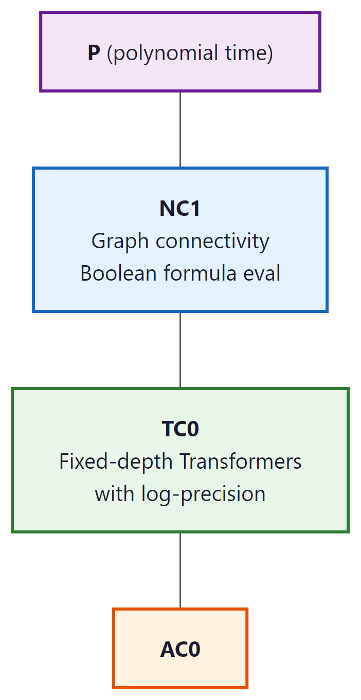
A foundational result by Merrill and Sabharwal (2023) shows that a fixed-depth Transformer with log-precision arithmetic (O(log n) bits per number, where n is the input length) can be simulated by TC⁰ circuits, and vice versa. $TC^{0}$ is the complexity class of problems solvable by constant-depth, polynomial-size threshold circuits.

This has concrete implications for what fixed-depth Transformers cannot do:

• Cannot solve problems that require counting precisely (e.g., determining if the number of 1s in a binary string is exactly equal to the number of 0s), because $TC^{0}$ cannot solve the "majority with equality" problem.
• Cannot solve inherently sequential problems like evaluating nested compositions of functions (e.g., computing $f(f(f(...f(x)...)))$ with n nested applications of an arbitrary function f).
• Cannot simulate a general-purpose Turing machine for an arbitrary number of steps, because $TC^{0}$ is strictly contained in P.

Figure 4.5.2: The complexity class hierarchy. Fixed-depth Transformers with log-precision arithmetic correspond to $TC^{0}$. Problems requiring sequential computation ($NC^{1}$ and above) are beyond their reach without additional mechanisms.

2.2 The Precision Assumption Matters

The $TC^{0}$ characterization assumes log-precision arithmetic: each number in the Transformer uses O(log n) bits. With unbounded precision (arbitrary-precision real numbers), a Transformer can simulate any Turing machine in polynomial time, making it trivially universal. This highlights that the precision of computation is a critical variable in the theoretical analysis.

In practice, Transformers use 16-bit or 32-bit floating point, which is somewhere between log-precision and unbounded precision. The practical implications of the theoretical results hold approximately: tasks requiring deep sequential reasoning are indeed harder for Transformers, even if the formal impossibility results rely on specific precision assumptions.

3. Limitations: What Transformers Struggle With

The theoretical results predict specific failure modes, and these predictions are borne out empirically. Here are the key categories of problems that fixed-depth Transformers find difficult:

3.1 Inherently Sequential Computation

Problems that require a long chain of dependent computation steps are hard for Transformers because each layer can only perform a constant amount of sequential work. The total sequential depth is the number of layers, typically 32 to 96. Tasks requiring more sequential steps than this (relative to the model's precision) become problematic.

Example: multi-step arithmetic. Computing ((3 + 7) * 2 - 4) / 3 requires evaluating operations in order. Each operation depends on the result of the previous one. A fixed-depth Transformer must either learn to parallelize this computation (difficult) or represent the intermediate results within a single forward pass (limited by depth).

3.2 Counting and Tracking State

Exact counting (e.g., "does this string have exactly 47 opening parentheses?") is difficult because log-precision attention scores cannot represent arbitrary integers precisely for long sequences. The model can approximate counting for small numbers but degrades as counts grow large.

3.3 Graph Reasoning

Problems like graph connectivity, shortest paths, and cycle detection require iterative algorithms that propagate information through the graph structure. A constant-depth Transformer can only propagate information a constant number of "hops" per layer, limiting its ability to reason about graph structures that require many hops.

4. Chain-of-Thought Extends Computational Power

This is perhaps the most practically important theoretical result. Chain-of-thought (CoT) reasoning, where the model generates intermediate reasoning steps before producing a final answer, fundamentally changes the computational model. We explore how to elicit CoT through prompt engineering techniques in Section 11.2, and how it shapes reasoning-focused models in Section 7.3. Instead of computing the answer in a single forward pass (constant depth), the model now performs computation proportional to the number of generated tokens.

4.1 CoT as Additional Computation Steps

When a Transformer generates T tokens of chain-of-thought reasoning, each token's generation involves a full forward pass through the model. The information from each token is fed back as input for the next, creating an effective sequential computation depth of $T \times N$ (tokens times layers). This is a fundamentally different computation than a single forward pass.

4.2 Why CoT Helps on Hard Problems

Consider the task of multiplying two large numbers, say 347 × 892. A single forward pass through a Transformer must compute this in constant depth, which the theory predicts is very difficult (large integer arithmetic is not in $TC^{0}$). But with CoT, the model can:

1. Break the multiplication into partial products (347 × 2, 347 × 90, 347 × 800)
2. Compute each partial product (one or two tokens of intermediate computation each)
3. Add the partial products (again, with intermediate steps)
4. Produce the final answer

Each individual step is simple enough for a single forward pass. The chain of thought provides the sequential depth that a single pass cannot.

4.3 Implications for LLM Design and Prompting

This theoretical framework has direct practical consequences:

• Prompting for reasoning: Asking the model to "think step by step" is not just about better prompts; it gives the model additional computational depth for problems that require it.
• Token budget matters: For hard reasoning tasks, limiting the model's output length directly limits its computational power. Longer chains of thought enable harder computations.
• Scratchpad training: Training models to use intermediate computation (reasoning tokens, scratchpads) is a way to extend their effective depth. This is the principle behind approaches like "thinking" tokens in some recent models.
• Verifiable vs. generative reasoning: The model's ability to generate a correct proof (step by step) may exceed its ability to directly produce the answer, because generation provides the sequential depth that direct answers require doing in a single pass.

5. Open Questions

Several fundamental questions remain open in this area:

• Practical expressiveness gaps: The theory identifies tasks that are provably hard for fixed-depth Transformers, but we lack a precise understanding of which real-world tasks are affected. Are there important NLP tasks that current models fail at specifically because of computational depth limitations?
• Depth vs. width tradeoffs: How does the tradeoff between model depth and model width affect the class of computable functions in practice? A very wide but shallow model versus a narrow but deep model may have qualitatively different capabilities.
• Implicit chain-of-thought: Can Transformers learn to perform internal "chain-of-thought" reasoning within their hidden layers, effectively using the residual stream as a scratchpad? Some evidence suggests this happens (intermediate layers performing identifiable reasoning steps), but the theory is not well developed.
• SSMs and expressiveness: How does the computational class of SSMs (Mamba, RWKV) compare to Transformers? SSMs have a recurrent structure that provides sequential depth, but they compress information into a fixed-size state. The expressiveness tradeoffs are not yet fully understood.

pip install numpy matplotlib torch

import numpy as np

def layer_norm(x, eps=1e-5):
 """Layer normalization: normalize each token's features to zero mean, unit variance."""
 mean = np.mean(x, axis=-1, keepdims=True)
 var = np.var(x, axis=-1, keepdims=True)
 return (x - mean) / np.sqrt(var + eps)

def feedforward(x, W1, b1, W2, b2):
 """Position-wise feedforward: Linear -> ReLU -> Linear."""
 hidden = np.maximum(0, x @ W1 + b1) # ReLU activation
 return hidden @ W2 + b2

# Test layer norm
x = np.random.randn(4, 16)
normed = layer_norm(x)
print(f"Before norm: mean={x[0].mean():.3f}, std={x[0].std():.3f}")
print(f"After norm: mean={normed[0].mean():.6f}, std={normed[0].std():.3f}")

def softmax(x, axis=-1):
 e_x = np.exp(x - np.max(x, axis=axis, keepdims=True))
 return e_x / np.sum(e_x, axis=axis, keepdims=True)

def self_attention(X, W_q, W_k, W_v, W_o, n_heads):
 """Multi-head self-attention (simplified, no mask)."""
 seq_len, d_model = X.shape
 d_head = d_model // n_heads
 Q, K, V = X @ W_q, X @ W_k, X @ W_v

 outputs = []
 for h in range(n_heads):
 q_h = Q[:, h*d_head:(h+1)*d_head]
 k_h = K[:, h*d_head:(h+1)*d_head]
 v_h = V[:, h*d_head:(h+1)*d_head]
 scores = q_h @ k_h.T / np.sqrt(d_head)
 weights = softmax(scores)
 outputs.append(weights @ v_h)

 return np.concatenate(outputs, axis=-1) @ W_o

def transformer_block(X, params):
 """One Transformer encoder block with Pre-LN residual connections."""
 # Sub-layer 1: Self-attention
 normed = layer_norm(X)
 attn_out = self_attention(normed, params["W_q"], params["W_k"],
 params["W_v"], params["W_o"], params["n_heads"])
 X = X + attn_out # Residual connection

 # Sub-layer 2: Feedforward
 normed = layer_norm(X)
 ff_out = feedforward(normed, params["W1"], params["b1"],
 params["W2"], params["b2"])
 X = X + ff_out # Residual connection
 return X

# Initialize parameters
d_model, d_ff, n_heads = 32, 64, 4
np.random.seed(42)
scale = 0.02
params = {
 "n_heads": n_heads,
 "W_q": np.random.randn(d_model, d_model) * scale,
 "W_k": np.random.randn(d_model, d_model) * scale,
 "W_v": np.random.randn(d_model, d_model) * scale,
 "W_o": np.random.randn(d_model, d_model) * scale,
 "W1": np.random.randn(d_model, d_ff) * scale,
 "b1": np.zeros(d_ff),
 "W2": np.random.randn(d_ff, d_model) * scale,
 "b2": np.zeros(d_model),
}

X = np.random.randn(6, d_model) # 6 tokens
output = transformer_block(X, params)
print(f"Input shape: {X.shape}")
print(f"Output shape: {output.shape}")
print(f"Residual preserved: input and output have same shape ✓")

import matplotlib.pyplot as plt

def sinusoidal_encoding(seq_len, d_model):
 """Generate sinusoidal positional encodings."""
 pe = np.zeros((seq_len, d_model))
 position = np.arange(seq_len)[:, np.newaxis]
 div_term = np.exp(np.arange(0, d_model, 2) * -(np.log(10000.0) / d_model))

 pe[:, 0::2] = np.sin(position * div_term)
 pe[:, 1::2] = np.cos(position * div_term)
 return pe

pe = sinusoidal_encoding(50, d_model)

fig, ax = plt.subplots(figsize=(10, 4))
im = ax.imshow(pe.T, cmap="RdBu", aspect="auto", interpolation="nearest")
ax.set_xlabel("Position")
ax.set_ylabel("Dimension")
ax.set_title("Sinusoidal Positional Encodings")
plt.colorbar(im, ax=ax)
plt.tight_layout()
plt.savefig("positional_encodings.png", dpi=150)
plt.show()

# Apply to input
X_with_pos = X + pe[:6] # Add positional info to 6 tokens
output_with_pos = transformer_block(X_with_pos, params)
print("Position-aware Transformer block output computed.")

import torch
import torch.nn as nn

# The same Transformer block in PyTorch
d_model, d_ff, n_heads, seq_len = 32, 64, 4, 6

encoder_layer = nn.TransformerEncoderLayer(
 d_model=d_model,
 nhead=n_heads,
 dim_feedforward=d_ff,
 batch_first=True,
 norm_first=True, # Pre-LN, matching our from-scratch version
)

x = torch.randn(2, seq_len, d_model) # batch of 2
output = encoder_layer(x)

print(f"PyTorch input shape: {x.shape}")
print(f"PyTorch output shape: {output.shape}")
print(f"\nParameter count: {sum(p.numel() for p in encoder_layer.parameters()):,}")
print(f"Components: self_attn, linear1, linear2, norm1, norm2")
print("\nFrom scratch: ~80 lines. PyTorch: ~10 lines. Same architecture.")

Bibliography

Yun, C., Bhojanapalli, S., Rawat, A.S., Reddi, S., Kumar, S. (2020). "Are Transformers universal approximators of sequence-to-sequence functions?" ICLR 2020.
Merrill, W. and Sabharwal, A. (2024). "The Expressive Power of Transformers with Chain of Thought." ICLR 2024.
Wei, C., Chen, Y., Ma, T. (2022). "Statistically Meaningful Approximation: a Case Study on Approximating Turing Machines with Transformers." NeurIPS 2022.