"BLEU, ROUGE, perplexity. The three letters that keep showing up at parties long after the host stopped inviting them."
Eval, Metric-Reference-Holder AI Agent
Classical ML metrics (BLEU, ROUGE, perplexity, classification precision/recall/F1) still anchor the LLM and RAG evaluation toolkit even in the era of LLM-as-judge: they are the cheap, deterministic, reproducible numbers your monitoring dashboard exposes and your paper has to report. This page is the lookup reference you reach for when an evaluation harness asks for "BLEU-4" and you need to remember what that means.
Prerequisites
This section assumes the train/validation/test split discussion from Section 0.1, the LLM evaluation framework from Section 42.1, and the language-model perplexity definition from Section 6.2.
For a comprehensive discussion of evaluation methodology, train/validation/test splits, and cross-validation, see Section 0.1: ML Basics: Features, Optimization & Generalization. For LLM-specific evaluation frameworks, see Section 42.1.
This page collects the most commonly referenced metrics in a single lookup location. For discussion of when and how to apply these metrics in practice, see the main text references above.
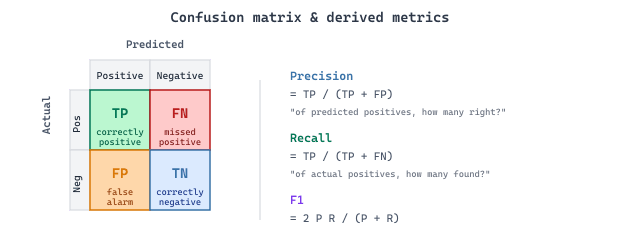
Classification Metrics
| Metric | Formula / Definition | Watch Out |
|---|---|---|
| Accuracy | Fraction of correct predictions | Misleading on imbalanced data (99% "not spam" baseline) |
| Precision | TP / (TP + FP) | High precision = few false positives |
| Recall | TP / (TP + FN) | High recall = few false negatives |
| F1 Score | $2 \cdot (P \cdot R) / (P + R)$ | Harmonic mean; balances precision and recall |
Language Generation Metrics
Algorithm: Corpus-level BLEU-N
Input:  candidate translations C = {c_1, .., c_S},
        reference sets R_s for each candidate c_s, n-gram order N (default 4),
        per-order weights w_n (default 1/N each)
Output: BLEU score in [0, 1]

  // 1. Modified n-gram precision (clip by max reference count to avoid spamming high-freq grams)
  For n = 1..N:
      num := 0;  den := 0
      For s = 1..S, for each n-gram g in c_s:
          count_c := count(g in c_s)
          count_max_ref := max over r in R_s of count(g in r)
          num := num + min(count_c, count_max_ref)
          den := den + count_c
      p_n := num / den

  // 2. Geometric mean of precisions
  GM := exp( sum_{n = 1..N} w_n * log p_n )

  // 3. Brevity penalty (discourages too-short outputs)
  c_total := total length of all candidates
  r_total := for each c_s, the closest-length reference; sum up r_s
  BP := 1                          if c_total > r_total
        exp(1 - r_total / c_total) if c_total <= r_total

  // 4. Final score
  BLEU := BP * GM
  Return BLEU

Properties.
   - Precision-based: counts how many candidate n-grams appear in the references.
   - "Modified" precision clips by the maximum reference count, preventing degenerate
     outputs that just repeat a common word.
   - Brevity penalty replaces the missing recall term; without it, an extremely short
     candidate could score 1.
   - BLEU-1 (unigrams) tracks lexical match; BLEU-4 tracks fluency by rewarding longer
contiguous matches.BP stands in for the missing recall term so that one-word candidates cannot game the score.Source: Papineni, Roukos, Ward, and Zhu, "BLEU: a Method for Automatic Evaluation of Machine Translation," ACL 2002 (aclanthology.org/P02-1040). The "sacre" variant (sacreBLEU, Post 2018) fixes tokenization and case so that scores are comparable across publications. BLEU correlates well with human judgments on machine translation but is known to underestimate paraphrase quality, which is why newer learned metrics (BERTScore, COMET, BLEURT) are now preferred for evaluating generative LLM outputs.
COMET and BLEURT are learned metrics: instead of counting n-gram overlap, they fine-tune a pretrained encoder to predict human quality scores directly. BLEURT pretrains BERT on synthetic perturbations with proxy signals, then fine-tunes on human ratings so it outputs a scalar quality estimate for a candidate against a reference. COMET encodes the source, the candidate, and the reference together with a multilingual encoder and regresses onto human direct-assessment scores, which lets it use the source sentence that surface metrics ignore. Because the scoring function is trained on human judgments rather than fixed, both track paraphrase and adequacy far better than BLEU, at the cost of a model dependency and sensitivity to the rating data they were trained on.
Algorithm: ROUGE-N (n-gram recall) and ROUGE-L (longest common subsequence)

------------------------------------------------------------------
ROUGE-N: n-gram recall against reference summary
------------------------------------------------------------------
Input:  candidate summary c, reference summary r, n-gram order n
Output: ROUGE-N in [0, 1]

  R_n := |n-grams(c) intersect n-grams(r)| / |n-grams(r)|
  // F-score variant uses precision and harmonic mean:
  P_n := |n-grams(c) intersect n-grams(r)| / |n-grams(c)|
  F_n := 2 P_n R_n / (P_n + R_n)

Common settings: ROUGE-1 (unigrams), ROUGE-2 (bigrams).

------------------------------------------------------------------
ROUGE-L: longest common subsequence
------------------------------------------------------------------
Input:  candidate token list c (length m), reference token list r (length n)
Output: ROUGE-L F-score

  // 1. Compute LCS length via dynamic programming
  LCS[0..m][0..n] := 0
  For i = 1..m, for j = 1..n:
      If c[i] == r[j]:
          LCS[i][j] := LCS[i-1][j-1] + 1
      Else:
          LCS[i][j] := max(LCS[i-1][j], LCS[i][j-1])
  L := LCS[m][n]

  // 2. LCS-based precision, recall, F (beta usually = 1)
  P_lcs := L / m
  R_lcs := L / n
  F_lcs := (1 + beta^2) * P_lcs * R_lcs / (R_lcs + beta^2 * P_lcs)
  Return F_lcs

Why ROUGE-L matters. The LCS does not require contiguous matches, so it rewards
in-order word overlap even when the candidate paraphrases connective words. This is
why ROUGE-L is the canonical metric for summarization, where surface paraphrase is
expected but topical content must align.O(mn) time and lets ROUGE-L credit paraphrases that BLEU's contiguous-match assumption would penalize.Source: Lin, "ROUGE: A Package for Automatic Evaluation of Summaries," ACL 2004 Workshop (aclanthology.org/W04-1013). The dominant ROUGE variants for LLM evaluation are ROUGE-1, ROUGE-2, and ROUGE-L; CNN/DailyMail leaderboards report all three. Like BLEU, ROUGE is surface-based: paraphrase-heavy LLM outputs can score lower than humans even when factually correct, which is why ROUGE has largely been supplemented (not replaced) by LLM-as-judge metrics for modern generative evaluation.
| Metric | Measures | Range | Used For |
|---|---|---|---|
| Perplexity | How surprised the model is by the data | 1 to ∞ (lower is better) | Language model evaluation |
| BLEU | N-gram overlap with reference text | 0 to 100 (higher is better) | Machine translation |
| ROUGE | Recall-oriented n-gram overlap | 0 to 1 (higher is better) | Summarization |
| BERTScore | Semantic similarity via embeddings | 0 to 1 (higher is better) | General text generation |
| METEOR | Alignment with synonyms and stemming | 0 to 1 (higher is better) | Machine translation, captioning |
# BLEU + ROUGE with Hugging Face evaluate library.
# BLEU measures n-gram precision (good for MT); ROUGE measures n-gram recall (good for summarization).
import evaluate

bleu = evaluate.load("bleu")
rouge = evaluate.load("rouge")

predictions = ["the cat sat on the mat",
               "transformers use self-attention"]
references  = [["a cat is sitting on the mat"],
               ["transformers rely on self-attention"]]

bleu_result  = bleu.compute(predictions=predictions, references=references)
rouge_result = rouge.compute(predictions=predictions,
                              references=[r[0] for r in references])

print(f"BLEU-4   : {bleu_result['bleu']:.3f}")
print(f"ROUGE-1  : {rouge_result['rouge1']:.3f}")
print(f"ROUGE-L : {rouge_result['rougeL']:.3f}")evaluate library. BLEU measures n-gram precision between prediction and reference, while ROUGE measures recall-oriented overlap. Both return scores between 0 and 1.Compute BLEU and ROUGE scores using Hugging Face's evaluate library.
# pip install evaluate rouge-score
import evaluate

bleu = evaluate.load("bleu")
result = bleu.compute(
    predictions=["The cat sat on the mat"],
    references=[["The cat is sitting on the mat"]]
)
print(f"BLEU: {result['bleu']:.3f}")

rouge = evaluate.load("rouge")
result = rouge.compute(
    predictions=["The cat sat on the mat"],
    references=["The cat is sitting on the mat"]
)
print(f"ROUGE-L: {result['rougeL']:.3f}")lang="en" parameter selects the appropriate pretrained model. The F1 score balances precision and recall of matched embedding tokens.Compute semantic similarity between generated and reference text using BERTScore.
# pip install evaluate bert-score
import evaluate

bertscore = evaluate.load("bertscore")
result = bertscore.compute(
    predictions=["The cat sat on the mat"],
    references=["The cat is sitting on the mat"],
    lang="en"
)
print(f"BERTScore F1: {result['f1'][0]:.3f}")BLEU and ROUGE measure surface-level text overlap, not meaning. A paraphrase that perfectly captures the intended meaning but uses different words will score poorly. This is why the field is increasingly moving toward LLM-as-judge evaluation (Chapter 29), where a powerful language model rates the quality of generated text. Human evaluation remains the gold standard for open-ended generation tasks, but it is expensive and slow.
Perplexity: A Deeper Look
Perplexity deserves special attention because it is the most commonly reported metric for language models. It is defined as:
Intuitively, a perplexity of $k$ means the model is as uncertain as if it were choosing uniformly among $k$ options at each step. A model with perplexity 10 is much more confident (and presumably more accurate) than one with perplexity 100. Code Fragment 42.12.4 below puts this into practice.
Algorithm: Sequence-level perplexity
Input:  tokenized sequence x = (x_1, .., x_N), autoregressive LM giving log p(x_i | x_{<i})
Output: perplexity PPL in [1, infinity)

  // 1. Average per-token negative log-likelihood (cross-entropy in nats)
  NLL := 0
  For i = 1..N:
      NLL := NLL + ( - log p(x_i | x_{<i}) )
  NLL_per_token := NLL / N

  // 2. Perplexity is the exponential of average NLL
  PPL := exp( NLL_per_token )
  Return PPL

Equivalences:
   PPL = 2^{H(x) / log 2}       (if NLL is measured in bits, base-2)
   PPL = exp( H(p_data, p_model) ) for a single long sequence
   PPL = (prod_i p(x_i | x_{<i}))^{-1/N}                  // geometric mean of 1/p
   Lower bound: PPL >= exp( H(data) )                    // Shannon entropy of the source
   Upper bound: PPL <= V                                  // vocabulary size (uniform model)

Interpretation. PPL = 32 means the model is, on average, as uncertain about the next
token as it would be if it had to choose uniformly among 32 equally-likely options.
A model with PPL = 8 is 4x more confident on average than one with PPL = 32.

Important caveats.
   - PPL is comparable only across models that share the same tokenization
     (BPE granularity changes N). For cross-tokenizer comparison, use "bits per byte"
     (Henighan et al. 2020) which divides bits by raw byte count, removing the
     tokenization confound.
   - PPL is well-defined only on text drawn from the same distribution the model was
trained on; OOD perplexity is a measurement of distribution shift, not quality.PPL <= V (vocabulary size) is the trivial uniform-model baseline; the lower bound PPL >= exp(H(data)) is the Shannon-entropy floor that no LM can beat on its training distribution.Perplexity is the standard intrinsic LM metric and the natural complement to cross-entropy: minimizing the training cross-entropy is exactly equivalent to minimizing perplexity on the training distribution. The Chinchilla and Kaplan scaling laws (Section 6.3) all express loss (test perplexity) as a power law in compute, parameters, and tokens. Cross-tokenizer comparisons should report "bits per byte" or "bits per character" instead, per Henighan et al., "Scaling Laws for Autoregressive Generative Modeling" (arXiv:2010.14701, 2020).
# PyTorch implementation
import torch
from transformers import AutoModelForCausalLM, AutoTokenizer

model_name = "gpt2"
tokenizer = AutoTokenizer.from_pretrained(model_name)
model = AutoModelForCausalLM.from_pretrained(model_name)

text = "The transformer architecture revolutionized natural language processing."
inputs = tokenizer(text, return_tensors="pt")

with torch.no_grad():
    outputs = model(**inputs, labels=inputs["input_ids"])
    perplexity = torch.exp(outputs.loss)
print(f"Perplexity: {perplexity.item():.2f}")GPT-2 (2019) achieved about 35 perplexity on WikiText-103. GPT-3 brought it below 20. Modern open models like Llama-3 push even lower. Each generation of models is, in a measurable sense, less surprised by human language. The trajectory suggests we are approaching fundamental limits of predictability in natural text.
- Supervised learning = labeled data; self-supervised = labels from structure; RL = learn from rewards.
- layer normalization is the standard LLM loss function. AdamW is the standard optimizer.
- Fight overfitting with weight decay, early stopping, and good data practices.
- Use perplexity for language models, F1 for classification, ROUGE for summarization.
- Automated metrics are useful but imperfect. Human evaluation and LLM-as-judge fill the gap.
- Always check for data contamination before trusting benchmark results.
You evaluate a fraud classifier on 10,000 transactions where 50 are fraud. Model A gets 99.0% accuracy and Model B gets 98.5% accuracy. Compute precision, recall, and F1 for each at the natural decision threshold, given that Model A flags 30 transactions (10 true fraud, 20 false) and Model B flags 100 transactions (45 true fraud, 55 false). Which model would you ship?
Answer Sketch
Model A: precision = 10/30 = 33%, recall = 10/50 = 20%, F1 = 0.25. Model B: precision = 45/100 = 45%, recall = 45/50 = 90%, F1 = 0.60. Ship Model B despite the lower accuracy. The accuracy metric is dominated by the 9950 negatives that both models trivially get right. On a 0.5% prevalence task, recall is what matters, and Model B catches 4.5x more fraud at a manageable false-positive volume.
For each task, pick the single most appropriate primary metric and explain why other metrics would mislead: (a) ranking the top-5 search results for an e-commerce query; (b) extractive QA answer span prediction; (c) abstractive news summarization; (d) a multi-label medical-image classifier with 200 labels and severe label imbalance.
Answer Sketch
(a) NDCG@5. Plain precision ignores rank order; clicks happen mostly on position 1. (b) Token-level F1 (the SQuAD-style metric). Exact match is too brittle for surface variants like "Paris" vs "Paris, France". (c) ROUGE-L plus a faithfulness metric. Accuracy is undefined for free-form text. (d) Macro F1 or AUC-PR per label. Micro F1 hides poor performance on rare labels by averaging over the common ones, masking dangerous misses in the medical setting.
What Comes Next
Continue to Section 5.1 (Platforms) for the next reference appendix in this collection.