"Premature optimization is the root of all evil, but failing to plan capacity is the root of all outages."
Adapted from Donald Knuth, Structured Programming, 1974
Compute planning starts before any GPU is rented: it is a sizing exercise driven by your serving SLO, model size, and traffic. This section walks the decisions that turn a chosen model into a hardware bill of materials and a deployment plan that survives real load.
Prerequisites
This section assumes familiarity with LLM API patterns from Section 11.1 and with latency-tail analysis from Section 44.3. The model-registry workflow is covered in detail later in the book.
Compute is the single largest variable cost in an LLM product. Get the planning wrong and you either burn the budget on idle GPUs or run out of capacity at the worst possible moment. This chapter shows how to size compute correctly: which GPUs match which workloads, when API calls are cheaper than self-hosting, how to forecast capacity for production traffic, and how to budget for the unpredictable cost spikes (long-context queries, agentic loops, model upgrades) that wreck plans built on average numbers.
The chapter assumes you have made the build-vs-buy decision from Chapter 63 and are now sizing the "build" side. If you are pure-API, much of this chapter is reference material rather than action items; you still need to understand the GPU tier story to predict your API costs, because providers price relative to their underlying hardware. This section opens with the basic vocabulary and the three workload categories that drive everything else.
57.1.1 The three workload categories
A 70-billion-parameter model in fp16 needs 140 GB just to load the weights, which means it does not fit on a single H100. Engineers usually discover this on a Friday afternoon, the day before a launch, and the resulting scramble to tensor-parallelize is responsible for a large fraction of all weekend overtime in modern AI startups.
Every LLM compute decision falls into one of three buckets. The categories matter because they have very different cost curves.
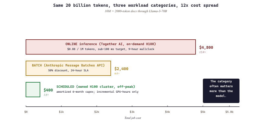
Take a single concrete task: process 10 million 2,000-token documents through Llama-3-70B for classification. Online inference on Together AI (sub-100ms latency target, on-demand H100s): roughly $4,800 at $0.88 per million tokens, completed in 9 hours. Batch inference on Anthropic's Message Batches API (24-hour SLA, no latency requirement): roughly $2,400 at half-price discount. Training-style scheduled batch on a reserved H100 cluster you own and amortize over 6 months: roughly $400 in incremental GPU-hours because the hardware was already paid for and ran during otherwise-idle nights. Same 20 billion tokens of work, three workload categories, 12x cost spread. The category you choose for a workload often matters more than the model you choose, and most teams discover this only after the third invoice.
- Training: pretraining or fine-tuning a model. Bursty, multi-hour-to-multi-day, throughput-bound. Hardware should be picked for FLOPs and memory-per-GPU. Idle cost is the dominant risk.
- Inference (online): serving production traffic with sub-second latency requirements. Steady-state, latency-bound, throughput per GPU varies with batch size. Hardware should be picked for memory bandwidth and prompt caching.
- Inference (batch): bulk processing where latency does not matter (overnight analytics, embedding generation, evaluation runs). Throughput-bound, often runs on spot or off-peak hardware. Costs can be 50-90% lower than online inference if you use the right discounts.
57.1.2 GPU tiers in 2026
The 2026 GPU landscape is broader than 2024's. The tiers you actually need to know:
- NVIDIA Blackwell B200 / B300: the new top tier, 180-192 GB HBM3e, ~8 TB/s bandwidth. ~$5-$8/hr in cloud markets through mid-2026. Used by the frontier labs for training; available for rental.
- NVIDIA GB200 NVL72: the rack-scale Blackwell system pairing 72 B200 GPUs with 36 Grace CPUs over NVLink Switch fabric. Sold as a single coherent unit and used by frontier labs (OpenAI, Anthropic, Meta) for the largest training runs of 2025-2026. Available through select clouds (CoreWeave, Azure, AWS) at multi-rack pricing.
- NVIDIA H100 / H200: the H100 (80 GB HBM3) was the 2023-25 workhorse; the H200 (141 GB HBM3e) is its memory-doubled successor. ~$2-$5/hr rental.
- NVIDIA A100 (80 GB): still widely available, still useful for inference of 70B models in 4-bit. ~$1-$2/hr.
- NVIDIA L40S / RTX 6000 Ada: 48 GB; the right inference GPU for 7B to 13B fp16 or 70B at 4-bit. ~$0.80-$1.50/hr.
- AMD MI355X: 288 GB HBM3e, ~6 TB/s. The largest-memory commodity GPU; pricing typically 70-80% of equivalent NVIDIA tier.
- Google TPU v6 Trillium and v7: Google's accelerators for the JAX / TPU ecosystem. Trillium (TPU v6e, GA mid-2024) delivers approximately 4.7x the FP8 throughput of TPU v5e per chip; the v7 generation (Ironwood, 2025) extended this further. Available only through Google Cloud Vertex AI / Pathways.
- Specialized accelerators: AWS Trainium 2 and Trainium 3 for Amazon-stack training, Groq LPU for very-low-latency inference, Cerebras WSE-3 (the wafer-scale chip with 900K cores), and Tenstorrent Blackhole for emerging non-CUDA workloads. These compete on specific axes (cost-per-token at scale for Trainium, sub-50ms latency for Groq, single-chip context for Cerebras) rather than on raw FLOPs.
- Consumer GPUs (RTX 5090, 4090): 24-32 GB. Right for development and small-volume inference.
57.1.3 Comparing the GPU options
| GPU | Memory | Bandwidth | Cloud $/hr | Best workload |
|---|---|---|---|---|
| NVIDIA B200 | 192 GB HBM3e | 8 TB/s | $5-$8 | Frontier training, big-model inference |
| NVIDIA H200 | 141 GB HBM3e | 4.8 TB/s | $3-$5 | 70B+ inference, mid-scale training |
| NVIDIA H100 | 80 GB HBM3 | 3.3 TB/s | $2-$4 | General-purpose 70B inference |
| NVIDIA A100 80GB | 80 GB HBM2e | 2 TB/s | $1-$2 | Cheap 70B 4-bit, dev / research |
| NVIDIA L40S | 48 GB GDDR6 | 0.86 TB/s | $0.80-$1.50 | 7B-13B fp16 inference |
| AMD MI355X | 288 GB HBM3e | 6 TB/s | $2-$4 | Largest-memory workloads |
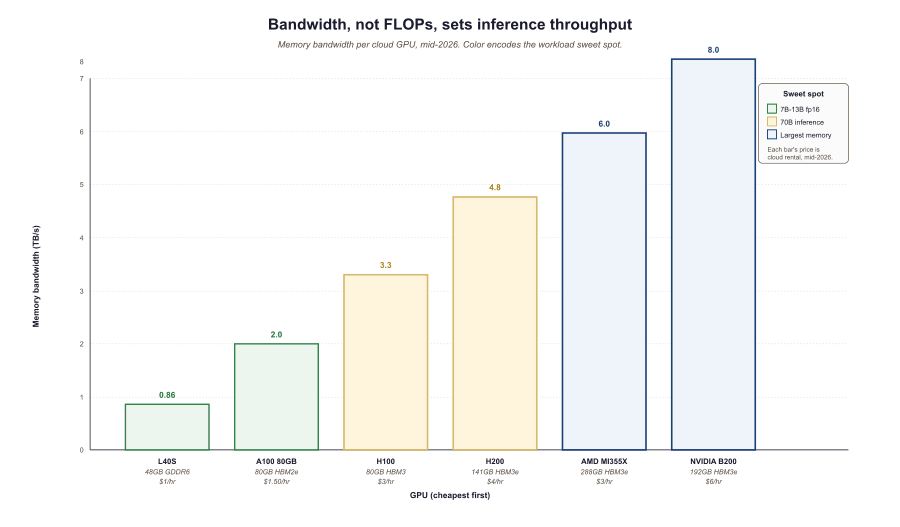
An H100 has roughly 2.5x the FLOPs of an A100 but only 1.6x the bandwidth. For inference, the bandwidth ratio is what predicts speedup, not the FLOPs ratio. The same logic flips on training: training is FLOPs-bound, and the H100 / B200's tensor-core advantage is what you are paying for. Match the GPU to the workload: bandwidth-heavy GPUs for inference, FLOPs-heavy GPUs for training. The "Making Deep Learning Go Brrrr" explainer remains the clearest walkthrough.
57.1.4 The capacity-planning timeline
Production capacity planning needs a three-horizon view. The thirty-day horizon is "what does my next month look like": traffic forecast, expected model upgrades, planned campaigns. The ninety-day horizon is "what does my next quarter look like": growth trajectory, infrastructure-cost commitments, reserved-capacity discounts. The twelve-month horizon is "what does next year look like": new hardware generations (Blackwell Ultra, Rubin), pricing changes, multi-cloud strategy. Plan for all three; commit only on the thirty-day horizon, hedge on the ninety, and watch on the twelve.
A 200K-token query costs 200x more compute than a 1K-token query. If your traffic distribution has a long tail of long-context requests (common in document QA, agent loops, code review), the average gives a useless capacity estimate. Plan against p95 and p99 token counts, not the mean. Token-count budgets per request are a useful guardrail; OpenAI Batch and Anthropic prompt-caching discounts can offset, but only if your traffic shape matches the discount terms.
Frontier-model providers offer aggressive discounts (30-60%) for reserved capacity commitments. The tempting move is to sign a one-year contract for cost certainty. The smarter move in 2026 is 30-day commits: model prices have dropped 50%+ year-over-year for the cheap tier (Gemini Flash, GPT-mini, Claude Haiku), and locking in last year's prices for a year is rarely the right bet. Most providers allow monthly commits without a multi-year contract.
57.1.5 A worked sizing derivation: from model to GPU count
The vocabulary above turns a model into a hardware shopping list only once we can answer the operative question: how many GPUs does a given model at a given traffic level actually need? Section 57.2 develops the full Pareto treatment, but the section would leave the reader stranded if it deferred every number. Here we derive a self-contained estimate from four inputs (model shape, GPU memory, a decode-latency target, and a target QPS) and plug in concrete numbers for one tier so the reader can reproduce the arithmetic.
The derivation has four steps. The first is the per-request memory footprint of the KV cache, which is what actually limits how many requests share a GPU. We reuse the part's KV-cache formula (the same one used for the 70B sizing in Section 57.4 and Exercise 27.14.3): for a context of $T$ tokens,
$$\text{KV}_{\text{req}} = 2 \cdot L \cdot H_{kv} \cdot d_{\text{head}} \cdot T \cdot b$$
where $L$ is the number of layers, $H_{kv}$ the number of key/value heads (under grouped-query attention this is smaller than the number of attention heads), $d_{\text{head}}$ the per-head dimension, $b$ the bytes per element (2 for fp16/bf16), and the leading factor of 2 counts the separate key and value tensors. The second step converts the GPU's free memory into a concurrency ceiling: after the weights are resident, the remaining memory divided by the per-request KV cost gives the maximum number of requests that can be in flight at once,
$$N_{\text{concurrent}} = \left\lfloor \frac{M_{\text{gpu}} - M_{\text{weights}}}{\text{KV}_{\text{req}}} \right\rfloor .$$
The third step turns concurrency into throughput. During autoregressive decode the server emits one token per request per forward pass, and a continuous-batching engine like vLLM runs a batch of $B \le N_{\text{concurrent}}$ requests through each pass in time $t_{\text{step}}$ (the per-token decode latency, memory-bandwidth bound, as established in Chapter 9). A request that emits $G$ output tokens therefore occupies a batch slot for $G \cdot t_{\text{step}}$ seconds, and the per-GPU request throughput is
$$\lambda_{\text{gpu}} = \frac{B}{G \cdot t_{\text{step}}} .$$
The fourth step divides the target traffic by per-GPU throughput and adds headroom, because a GPU planned to 100% utilization has no slack for the long-context tail (Section 57.1.4) or for traffic bursts. With a utilization target $u$ (a headroom factor; $u = 0.7$ leaves 30% slack),
$$N_{\text{gpu}} = \left\lceil \frac{\text{QPS}_{\text{target}}}{u \cdot \lambda_{\text{gpu}}} \right\rceil .$$
Consider one concrete tier: an 8B model (Llama-3.1-8B: $L = 32$ layers, $H_{kv} = 8$ KV heads under GQA, $d_{\text{head}} = 128$) served in bf16 on a single 80 GB H100, at a context of $T = 8{,}000$ tokens, with $G = 256$ output tokens per request and a target of 50 QPS. The weights take $8 \times 10^9 \cdot 2 = 16$ GB. The per-request KV cache is
$$\text{KV}_{\text{req}} = 2 \cdot 32 \cdot 8 \cdot 128 \cdot 8000 \cdot 2 = 1.05 \times 10^9 \ \text{bytes} \approx 0.98 \ \text{GB} .$$
The free memory after weights is $80 - 16 = 64$ GB, so $N_{\text{concurrent}} = \lfloor 64 / 0.98 \rfloor = 65$ requests. Suppose the engine runs a steady decode batch of $B = 48$ (below the ceiling, leaving room for prefill and fragmentation) at a per-token decode latency of $t_{\text{step}} = 18$ ms, a representative bandwidth-bound figure for an 8B model on an H100. Then each request, emitting 256 tokens, holds its slot for $256 \cdot 0.018 = 4.6$ s, and
$$\lambda_{\text{gpu}} = \frac{48}{256 \cdot 0.018} = \frac{48}{4.6} \approx 10.4 \ \text{req/s} .$$
At a utilization target of $u = 0.7$, one H100 sustains $0.7 \cdot 10.4 \approx 7.3$ QPS of usable throughput, so the fleet needs
$$N_{\text{gpu}} = \left\lceil \frac{50}{7.3} \right\rceil = \lceil 6.85 \rceil = 7 \ \text{H100s} .$$
Seven GPUs for 50 QPS of an 8B model at 8K context: the number is dominated by the decode-latency term, not the memory term (the memory ceiling of 65 concurrent requests is never the binding constraint here, because the batch the latency budget allows is far smaller). That is the typical regime for short-to-medium contexts, and it is why Section 57.4 spends its effort on batching and KV-cache reuse rather than on raw memory. The relationship inverts at very long context, where $\text{KV}_{\text{req}}$ grows linearly in $T$ and the concurrency ceiling becomes binding.
Code Fragment 1 packages this derivation as a runnable sizing function so the reader can vary the model shape, context length, and latency target and watch the GPU count move.
# GPU sizing estimate for online LLM serving.
# Chains the four steps from the derivation above:
# KV-cache per request -> concurrency ceiling -> per-GPU throughput -> fleet size.
import math

def gpus_needed(
    params: float,        # model parameter count, e.g. 8e9
    layers: int,          # transformer layers L
    kv_heads: int,        # key/value heads H_kv (GQA-aware)
    head_dim: int,        # per-head dimension d_head
    context: int,         # context length T in tokens
    out_tokens: int,      # generated tokens per request G
    gpu_mem_gb: float,    # GPU memory budget M_gpu
    decode_ms: float,     # per-token decode latency t_step in ms
    batch: int,           # steady decode batch B
    target_qps: float,    # target queries per second
    bytes_per_param: int = 2,  # bf16 weights
    util: float = 0.7,    # headroom factor u
) -> int:
    weights_gb = params * bytes_per_param / 1e9
    kv_req_gb = 2 * layers * kv_heads * head_dim * context * 2 / 1e9
    free_gb = gpu_mem_gb - weights_gb
    n_concurrent = math.floor(free_gb / kv_req_gb)
    eff_batch = min(batch, n_concurrent)  # cannot batch past the memory ceiling
    per_request_s = out_tokens * decode_ms / 1000
    lambda_gpu = eff_batch / per_request_s  # requests per second per GPU
    return math.ceil(target_qps / (util * lambda_gpu))

n = gpus_needed(
    params=8e9, layers=32, kv_heads=8, head_dim=128,
    context=8000, out_tokens=256, gpu_mem_gb=80,
    decode_ms=18, batch=48, target_qps=50,
)
print(f"GPUs needed: {n}")decode_ms or raising batch drops the count, while raising context eventually makes the memory ceiling (n_concurrent) the binding term. It is a planning estimate, not a load test: Section 57.2 refines it with prefill cost, the latency-throughput Pareto frontier, and measured per-token latency curves.57.1.6 What comes next
Section 57.2 takes up the sizing math itself in full: given a model, a target latency, and a target QPS, how many GPUs do you actually need once prefill cost and the latency-throughput frontier are accounted for? Sections 46.3 and 46.4 cover the cloud-provider comparison and the breakeven analysis between API and self-hosting that closes Chapter 57.
Sizing starts with planning, but the next operational question is how to integrate the compute plan with the rest of your enterprise: data flow, identity, change management. Continue to Section 57.2: Enterprise Integration Patterns for LLM Systems.