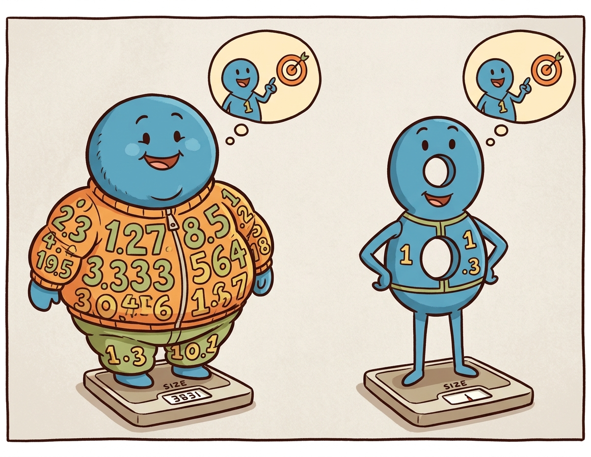
Quantization is the fine art of convincing a 70-billion-parameter model that it never really needed all those decimal places. Surprisingly, it usually agrees.
Quant, Precision Trimming AI Agent
Why quantize? A 70B-parameter model stored in FP16 requires approximately 140 GB of GPU memory just for the weights. That exceeds the capacity of even the largest single GPU (the A100 has 80 GB, the H100 has 80 GB). Quantization compresses weights from 16-bit or 32-bit floating point down to 8-bit, 4-bit, or even lower precision integers. A 4-bit quantized 70B model fits in roughly 35 GB, making it servable on a single GPU. This same principle underlies QLoRA, which combines 4-bit quantization with parameter-efficient fine-tuning. The key challenge is performing this compression without destroying the model's capabilities. Building on the distributed training techniques from Section 6.6 that addressed the training-time memory problem, this section covers the mathematics of quantization, the major algorithms (GPTQ, AWQ, bitsandbytes), and practical techniques for evaluating the quality tradeoff.
Prerequisites
This section assumes understanding of floating-point number representation and Section 0.3 tensor operations from Section 0.2. The matrix multiplication concepts from Section 3.1 (attention computations) are essential for understanding where quantization is applied.
Intuition: Quantization is like reducing the color depth of an image. A photo in 24-bit color uses 16.7 million distinct colors. Reduce it to 8-bit (256 colors) and the image is 3x smaller with barely visible quality loss. Reduce further to 4-bit (16 colors) and you start to see artifacts, but the image remains recognizable. Model quantization works the same way: reducing the precision of each weight from 16-bit to 4-bit shrinks the model 4x, with a small and often acceptable quality tradeoff.
9.1.1 Why Inference Is Expensive
NF4 ("4-bit NormalFloat") is the QLoRA paper's signature trick and a beautiful example of distribution-aware quantization. The insight: pretrained weight tensors are empirically near-Gaussian with mean 0 and known variance. Integer quantization spends equal precision on values that almost never occur (the tails) and values that occur constantly (near zero). NF4 instead places its 16 quantization levels at the quantiles of a standard normal, so each level carries equal probability mass. This is information-theoretically optimal for Gaussian data and beats INT4 by 0.5-1.0 perplexity points on the same bit budget. The lesson generalizes: every quantization scheme is implicitly a prior on the value distribution.
BF16 has the same exponent width as FP32 (8 bits) but a truncated mantissa (7 bits vs FP16's 5 exponent + 10 mantissa). This is not arbitrary: in mixed-precision training the dangerous failure mode is gradient underflow into zero, not precision loss in the high-order bits. BF16 preserves the FP32 dynamic range, so loss scaling (the awkward hack required for FP16) becomes unnecessary. FP16's wider mantissa would only matter if activations were already near the same magnitude; in transformers they span many orders of magnitude across layers, so range beats precision. This is why every modern LLM training pipeline since GPT-NeoX uses BF16.
The decision to quantize is rarely purely technical. For the cost/quality tradeoff framed as a build-vs-buy decision (self-host quantized vs API), see Section 11.1: LLM API Landscape and Pricing and Section 57.1: Compute Planning.
A finance startup quantized their fine-tuned Llama-3 70B model from FP16 to INT4 to fit on a single A100. Throughput tripled. Then their evaluation harness flagged a 22-point drop on GSM8K (grade-school math). Investigation showed that numerical reasoning relies on precise intermediate activations; INT4 quantization introduced enough noise in the residual stream to flip digits during multi-step arithmetic. Lesson: quantization quality is task-dependent. Always evaluate on the tasks that matter before shipping a quantized model, not just on aggregate benchmarks. The fix here was per-channel quantization on the FFN layers and FP8 on the attention output, recovering 18 of the 22 points.
Team G deployed an INT4 quantized version of their fine-tuned 13B model in production. End-to-end accuracy on their internal eval dropped 1pp, acceptable. Two weeks in, math-heavy customer queries showed 18pp accuracy drop. Internal eval had under-sampled math. Root cause: INT4 quantization preserves average-case behavior but destroys precision for arithmetic where small numerical errors compound across reasoning steps. Fix: stratified eval covering math, code, reasoning, and other arithmetic-sensitive categories before any quantization-level deployment. Use INT8 or BF16 for arithmetic-heavy queries (route by classifier). Lesson: aggregate accuracy metrics hide subgroup-specific regressions; always stratify your eval by capability category.
During autoregressive generation, the model produces one token at a time. Each token requires a full forward pass through every layer, reading all model weights from GPU memory. For a 70B model in FP16, this means transferring 140 GB of data per token through the memory bus. On an A100 with 2 TB/s memory bandwidth, merely reading the weights takes about 70 milliseconds. The actual computation (matrix multiplications) takes far less time. This makes LLM inference memory-bandwidth-bound, not compute-bound. The models most commonly quantized in practice are the open-weight families surveyed in Section 7.3.
Quantization helps in two complementary ways. First, smaller weights mean less data to transfer from memory, directly improving throughput. Second, smaller weights let the entire model fit on fewer (or smaller) GPUs, slashing hardware costs (a critical factor for the deployment scenarios discussed in Section 13.3). A model quantized to 4-bit occupies one quarter of the original memory, so weight transfer is roughly 4x faster.
The memory footprint shrinks 4x, but throughput often grows by 2 to 3x, not 4x. The reason: dequantization back to FP16 for the matrix multiply is not free, and the activations are still in higher precision (W4A16 means 4-bit weights but 16-bit activations). End-to-end speedup also depends on whether the workload is memory-bandwidth-bound (single user, decode) or compute-bound (batched prefill); only the first regime sees the full 4x. Always benchmark on your actual workload shape before promising users a "4x speedup."
Why models survive losing precision. Neural network weights are inherently approximate: they are the result of a stochastic optimization process that could have converged to slightly different values with a different random seed. Most individual weights can be perturbed by a small amount without measurably changing the model's output. Quantization exploits this tolerance by rounding each weight to the nearest value on a coarse grid. The precision chain from training to deployment typically goes FP32 (master weights) to BF16 (inference baseline) to FP8 or INT4 (optimized inference), with each step trading numerical precision for speed and memory savings. This is why the same principle works both during training (mixed-precision training in Section 6.6) and during inference: the weights were never exact to begin with, so rounding them further changes very little.
Who: An independent AI researcher wanting to run Llama-3.1 70B locally for private experimentation on a workstation with two RTX 4090 GPUs (24 GB VRAM each, 48 GB total).
Situation: The FP16 model required 140 GB of VRAM, far exceeding the available 48 GB. Even with tensor parallelism across both GPUs, the model could not fit.
Problem: The researcher needed the 70B model's quality for their NLP research benchmarks; the 8B model was insufficient for their experiments on complex reasoning tasks.
Dilemma: GPTQ 4-bit quantization would shrink the model to roughly 35 GB (fits in 48 GB with room for KV cache), but the researcher worried about quality degradation on their specific evaluation suite. AWQ claimed better quality preservation but was slower to quantize.
Decision: They compared GPTQ-4bit, AWQ-4bit, and bitsandbytes NF4 on their evaluation suite of 1,000 reasoning questions, ultimately selecting AWQ-4bit.
How: Using a pre-quantized AWQ model from Hugging Face, they loaded it across both GPUs using device_map="auto" in the Transformers library, served through a local vLLM instance.
Result: AWQ-4bit retained 96.8% of the FP16 model's accuracy on their benchmark (vs. 95.1% for GPTQ and 96.2% for NF4). The model fit comfortably in 36 GB, leaving 12 GB for KV cache, enabling a 4K context window at batch size 1. Generation speed reached 18 tokens/second.
Lesson: 4-bit quantization makes 70B-class models accessible on consumer GPUs with minimal quality loss. Always benchmark quantized models on your specific tasks, as quality degradation varies across domains and methods.
The practical example above shows quantization in action, but to choose wisely between methods (and debug issues when they arise), you need to understand what is happening mathematically. How exactly do we compress 16-bit or 32-bit floating point numbers into 4-bit integers without destroying the model?
9.1.2 Quantization Mathematics
Quantization is the art of convincing a model that it does not actually need 32 bits of precision per weight. In practice, most models barely notice the difference between 16-bit and 4-bit weights, which is the neural network equivalent of discovering that expensive wine and mid-range wine taste the same in a blind test.
9.1.2.1 Absmax (Symmetric) Quantization
The simplest quantization scheme maps a floating-point tensor to integers using only a scale factor. For an $n$-bit signed integer representation with range [$-2^{n-1}$, $2^{n-1}-1$], the quantization formula is:
Each value is then divided by this scale and rounded to the nearest integer:
To recover an approximation of the original values, the quantized integers are multiplied back by the scale:
Here, $X$ is the original floating-point tensor, $X_{q}$ is the quantized integer tensor, and $\hat{X}$ is the dequantized approximation. The zero point in the floating-point space always maps to integer zero, which is why this scheme is called symmetric. It works well when values are roughly centered around zero, which is typically true for neural network weights.
A worked example makes the round-trip concrete. Consider quantizing a small weight tensor to INT8 (n=8, range [−127, 127]):
# Numeric example: absmax (symmetric) INT8 quantization round-trip
import torch
X = torch.tensor([0.3, -0.5, 0.1, 0.8, -0.2])
n_bits = 8
scale = X.abs().max() / (2**(n_bits - 1) - 1) # 0.8 / 127 = 0.0063
X_q = torch.round(X / scale).clamp(-127, 127).to(torch.int8)
X_hat = X_q.float() * scale # dequantize
print(f"Original: {X.tolist()}")
print(f"Scale: {scale:.6f}")
print(f"Quantized: {X_q.tolist()}")
print(f"Dequantized: {[round(v, 4) for v in X_hat.tolist()]}")
print(f"Max error: {(X - X_hat).abs().max():.6f}")# Example 3: Quantizing with AWQ using the autoawq library
from awq import AutoAWQForCausalLM
from transformers import AutoTokenizer
model_name = "meta-llama/Llama-3.1-8B-Instruct"
quant_path = "./llama-8b-awq-4bit"
# Load model for quantization
model = AutoAWQForCausalLM.from_pretrained(model_name)
tokenizer = AutoTokenizer.from_pretrained(model_name)
# Configure AWQ
quant_config = {
"zero_point": True, # Use asymmetric quantization
"q_group_size": 128, # Group size
"w_bit": 4, # 4-bit weights
"version": "GEMM", # Optimized GEMM kernels
}
# Quantize (uses calibration data internally)
model.quantize(tokenizer, quant_config=quant_config)
model.save_quantized(quant_path)
tokenizer.save_pretrained(quant_path)
print(f"AWQ model saved to {quant_path}")
print(f"Original size: ~16 GB (FP16)")
print(f"Quantized size: ~4.5 GB (INT4)")9.1.2.2 Zero-Point (Asymmetric) Quantization
In practice, PyTorch provides built-in quantization primitives that handle scale computation, rounding, and clamping in a single call:
# Library shortcut: PyTorch built-in symmetric quantization
import torch
X = torch.tensor([0.3, -0.5, 0.1, 0.8, -0.2])
scale = X.abs().max() / 127
X_q = torch.quantize_per_tensor(X, scale=scale.item(), zero_point=0, dtype=torch.qint8)
print(f"Quantized: {X_q.int_repr().tolist()}")
print(f"Dequantized: {X_q.dequantize().tolist()}")quantize_per_tensor handles the full round-trip in a single call, matching the manual implementation above.When the tensor values are not symmetric around zero (common for activations, which often have a positive bias), asymmetric quantization adds a zero-point offset:
The zero-point offset shifts the integer range so that floating-point zero maps to a specific integer value:
The quantized value then combines the scaled rounding with this offset:
This maps the full range [min(X), max(X)] onto the unsigned integer range [0, 2n−1]. Dequantization reverses the process: $\hat{X} = (X_{q} - zero_{point}) \times scale$. The extra zero-point parameter adds slight overhead but significantly reduces quantization error for skewed distributions.
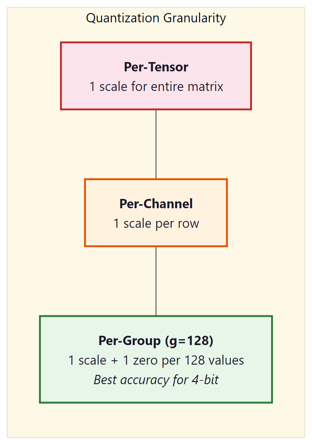
9.1.2.3 Granularity: Per-Tensor, Per-Channel, Per-Group
The scale (and zero-point) can be computed at different granularities:
- Per-tensor: One scale for the entire weight matrix. Simplest and fastest, but the largest outlier in the tensor dominates the scale for all values.
- Per-channel: One scale per output channel (row of the weight matrix). Common for INT8 quantization. Each row gets its own range, reducing the impact of outliers.
- Per-group: One scale per group of $g$ consecutive values (typically $g$ = 128). This is the standard for 4-bit quantization (GPTQ, AWQ, bitsandbytes). The overhead of storing extra scales is small (one FP16 scale per 128 INT4 values adds only 0.125 bits per value), but the accuracy improvement is substantial.
9.1.3 Data Types for Quantization
| Data Type | Bits | Range | Use Case |
|---|---|---|---|
| FP32 | 32 | ±3.4 × 1038 | Training (master weights) |
| FP16 / BF16 | 16 | ±65504 / ±3.4 × 1038 | Standard inference, mixed-precision training |
| FP8 (E4M3) | 8 | ±448 | Hopper GPU inference, training forward pass |
| FP8 (E5M2) | 8 | ±57344 | Training backward pass (wider range) |
| INT8 | 8 | −128 to 127 | Weight + activation quantization |
| INT4 | 4 | −8 to 7 | Weight-only quantization (GPTQ, AWQ) |
| NF4 | 4 | 16 quantile levels | bitsandbytes / QLoRA |
9.1.3.1 NF4: Normal Float 4-bit
NF4 is a special 4-bit data type designed by Tim Dettmers for use in QLoRA. The key insight is that neural network weights are approximately normally distributed. Instead of using uniformly spaced quantization levels (as standard INT4 does), NF4 places its 16 quantization levels at the quantiles of the standard normal distribution. This means each of the 16 bins captures approximately the same probability mass, making NF4 information-theoretically optimal for normally distributed data.
Concretely, given a standard normal CDF $\Phi$ and 16 desired levels, the negative branch places level $i$ at the quantile
with the positive branch defined symmetrically and the whole code book rescaled so that the extreme values are exactly $\pm 1$. Per group of $g = 64$ weights the quantizer first normalises by the absolute maximum, $\tilde{w} = w / \max_j |w_j|$, then picks the nearest entry in the 16-level code book:
Standard INT4 wastes quantization levels in low-density tails and crowds them in the high-density center. NF4 fixes this by spacing levels at normal quantiles. The 16 NF4 values are precomputed: {−1.0, −0.6962, −0.5251, −0.3949, −0.2844, −0.1848, −0.0911, 0.0, 0.0796, 0.1609, 0.2461, 0.3379, 0.4407, 0.5626, 0.7230, 1.0}.
# Load a 7B model with NF4 weights using bitsandbytes (the QLoRA recipe)
from transformers import AutoModelForCausalLM, BitsAndBytesConfig
import torch

nf4_cfg = BitsAndBytesConfig(
    load_in_4bit=True,
    bnb_4bit_quant_type="nf4",          # 16 quantile-spaced levels
    bnb_4bit_use_double_quant=True,     # quantise the scales too
    bnb_4bit_compute_dtype=torch.bfloat16,
)
model = AutoModelForCausalLM.from_pretrained(
    "meta-llama/Llama-3.1-8B-Instruct",
    quantization_config=nf4_cfg,
    device_map="auto",
)
print(model.get_memory_footprint() / 1e9, "GB")
# Output: ~5.4 GB on disk + ~0.5 GB for double-quantised scalesbitsandbytes. The 16 GB FP16 checkpoint shrinks to roughly 5.4 GB, leaving room for a 24 GB GPU to host both the model and a long KV cache.Suppose a per-group block of 64 weights is drawn from $\mathcal{N}(0, 1)$. Symmetric INT4 places 16 levels uniformly on $[-1, 1]$ with spacing $\Delta = 2/15 \approx 0.133$, so the worst-case reconstruction error per weight is roughly $\Delta / 2 \approx 0.067$. NF4 instead spaces levels at normal quantiles, with the tightest spacing near zero (≈ 0.08) and the widest near $\pm 1$ (≈ 0.27), matching the density of the weight distribution. On the 8B Llama 2 base model, this swap drops perplexity on WikiText-2 from 5.83 (uniform INT4) to 5.50 (NF4) at the same 4-bit memory budget, while plain FP16 sits at 5.47 (QLoRA paper, Table 2). NF4 recovers roughly 90% of the FP16 to INT4 gap at zero extra storage cost.
9.1.3.2 FP8 Inference on Hopper GPUs
FP8 (8-bit floating point) has emerged as the sweet spot for production inference on NVIDIA's Hopper architecture (H100, H200) and its successors. Unlike INT8 quantization, which requires calibration to determine scale factors and zero points, FP8 preserves the floating-point format with an exponent and mantissa. Two FP8 variants exist: E4M3 (4 exponent bits, 3 mantissa bits, range ±448) optimized for the forward pass, and E5M2 (5 exponent bits, 2 mantissa bits, range ±57344) designed for gradients during training. For inference, E4M3 is the standard choice because it offers better precision within the value ranges typical of activations and weights.
The Hopper Tensor Cores provide native hardware support for FP8 matrix multiplications, delivering roughly 2x the throughput of FP16/BF16 operations on the same hardware. This is not a software emulation; the H100 includes dedicated FP8 datapaths that process twice as many elements per clock cycle compared to their 16-bit counterparts. The result is that an FP8 model on a single H100 can match or exceed the throughput of the same model in FP16 on two H100s, effectively halving infrastructure costs.
The quality impact of FP8 inference is remarkably small. For models with 8 billion parameters and above, FP8 quantization typically introduces less than 0.1% perplexity degradation, a difference well within the noise of most benchmark evaluations. This is because 8 bits of floating-point precision are sufficient to represent the value distributions found in transformer weights and activations. Smaller models (under 3B parameters) may show slightly more sensitivity, but the effect remains modest.
In practice, FP8 inference is straightforward to enable in modern serving frameworks:
# vLLM with FP8 quantization on H100
from vllm import LLM, SamplingParams
llm = LLM(
    model="meta-llama/Llama-3.1-70B-Instruct",
    quantization="fp8", # Enable FP8 weight quantization
    dtype="float16", # Compute dtype for non-quantized ops
    tensor_parallel_size=4,
)
# TensorRT-LLM: FP8 is enabled during engine build
# trtllm-build --model_dir ./llama-70b \
# --output_dir ./engines/fp8 \
# --dtype float16 \
# --quantization fp8 \
# --tp_size 4FP8 inference requires Hopper (SM90) or newer GPUs. On Ampere (A100) and older hardware, INT8 or INT4 quantization remains the best option for reducing memory footprint and increasing throughput. If you are deploying on cloud providers, look for H100 or H200 instance types to take advantage of native FP8 support.
Compute the model weights memory footprint for an 8B-parameter LLM stored as FP16, INT8, INT4, and NF4. Then determine which of those fit in a 24 GB consumer GPU (RTX 4090) once you reserve 8 GB for the KV cache and activations.
Answer Sketch
FP16: 8B x 2 bytes = 16 GB. INT8: 8B x 1 byte = 8 GB. INT4 / NF4: 8B x 0.5 bytes = 4 GB. With 16 GB available for weights, FP16 just barely fits (no headroom for the KV cache), INT8 leaves 8 GB free, and INT4 leaves 12 GB. Real workloads on RTX 4090 typically choose INT4 or NF4 to leave room for a longer context window.
You quantize a 7B model with symmetric INT8 weights and observe a 0.6-point drop on MMLU (from 64.2 to 63.6). Then you switch to GPTQ INT4 and the drop grows to 1.8 points. Explain why GPTQ INT4 still ships in production even with the larger drop, and identify one workload where you would refuse to go below INT8.
Answer Sketch
INT4 halves memory vs INT8 and roughly doubles token throughput on memory-bound workloads, which pays for the 1.8-point quality drop in most chat use cases. Refuse INT4 when (a) the model is used for high-stakes tool selection or code generation where small accuracy drops compound, or (b) outputs are graded against a reference rubric where the drop crosses a release threshold. Math benchmarks (GSM8K) typically drop harder than MMLU under INT4 and are a useful guardrail.
What's Next?
In the next part of this section, Section 9.2: Quantization: Algorithms, Practice & QAT, why inference is expensive, the mathematics of quantization, and the data types (int8, int4, nf4, fp8) used to store quantized weights.