"A dashboard with twelve charts is a dashboard nobody reads. A dashboard with three charts is a dashboard somebody pages on at 3 AM. Choose."
A Dashboard-Designing AI Agent
Evaluating LLMs requires more than tracking a single loss metric. You need dashboards that surface generation quality, latency distributions, cost per request, safety violations, and drift over time. This section covers how to build LLM-specific evaluation dashboards in W&B and MLflow, instrument production systems for observability, track prompt-level metrics, and set up alerting for quality regressions. The techniques here connect experiment-time evaluation (covered in Section 19.13 (Libraries & Frameworks)) with production monitoring to create a continuous feedback loop.
Prerequisites
This section assumes familiarity with the model registry workflow from Section 44.1 and with evaluation metrics from Section 42.1 (BLEU, ROUGE, BERTScore, LLM-as-judge). Familiarity with prompt engineering from Section 12.1 helps when designing prompt-level dashboard widgets.
44.2.1 LLM Evaluation Metrics
Traditional ML models produce predictions easy to score: accuracy, F1, AUC. LLM outputs are free-form text, which needs a richer set of evaluation metrics. A comprehensive evaluation dashboard should track metrics across several dimensions.
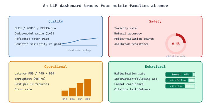
Quality metrics include BLEU, ROUGE, BERTScore, and judge-model scores. Safety metrics capture toxicity rates, refusal accuracy, and policy violation counts. Operational metrics track latency (P50, P95, P99), throughput (tokens per second), and cost (dollars per 1,000 requests). Behavioral metrics measure hallucination rates, instruction-following accuracy, and format compliance. Logging all of these during evaluation runs creates the foundation for a useful dashboard.
import wandb
import numpy as np
from datetime import datetime

def run_llm_evaluation(model, eval_dataset, run_name="eval"):
    """Run a comprehensive LLM evaluation and log to W&B."""
    run = wandb.init(
        project="llm-eval-dashboard",
        name=run_name,
        job_type="evaluation",
        config={
            "model": model.name,
            "eval_dataset": eval_dataset.name,
            "num_examples": len(eval_dataset),
            "timestamp": datetime.now().isoformat(),
        },
    )

    results = {"quality": [], "latency_ms": [], "tokens_out": []}
    safety_violations = 0
    format_failures = 0

    for example in eval_dataset:
        output, latency, token_count = model.generate_timed(example.prompt)

        # Score quality with a judge model
        quality = judge_model.score(
            prompt=example.prompt,
            response=output,
            reference=example.reference,
        )
        is_safe = safety_classifier.check(output)
        follows_format = check_output_format(output, example.expected_format)

        results["quality"].append(quality)
        results["latency_ms"].append(latency * 1000)
        results["tokens_out"].append(token_count)
        if not is_safe:
            safety_violations += 1
        if not follows_format:
            format_failures += 1

    # Log aggregate metrics
    wandb.log({
        "eval/quality_mean": np.mean(results["quality"]),
        "eval/quality_p25": np.percentile(results["quality"], 25),
        "eval/quality_median": np.median(results["quality"]),
        "eval/latency_p50": np.percentile(results["latency_ms"], 50),
        "eval/latency_p95": np.percentile(results["latency_ms"], 95),
        "eval/latency_p99": np.percentile(results["latency_ms"], 99),
        "eval/safety_violation_rate": safety_violations / len(eval_dataset),
        "eval/format_compliance": 1 - format_failures / len(eval_dataset),
        "eval/avg_tokens_out": np.mean(results["tokens_out"]),
    })

    run.finish()
return resultsNotice we log percentiles, not just means. For latency, P99 matters far more than the average because it sets worst-case user experience. For quality, the P25 value reveals how the model performs on its hardest examples, which is often more actionable than the mean.
Mean quality scores hide bimodal distributions. A model that scores 0.95 on 80% of examples and 0.20 on the remaining 20% has a mean of 0.80, which looks acceptable. But one in five users gets a terrible response. Always log the full distribution (P25, median, P75, P99) and inspect the bottom quartile to catch these failure modes.
44.2.2 Prediction Tables and Qualitative Review
Aggregate metrics cannot tell you why a model fails. Prediction tables log individual examples so that you (or your domain experts) can review actual model outputs and identify patterns in failures.
import wandb

def log_prediction_table(model, eval_dataset, max_rows=200):
    """Log a browsable table of model predictions to W&B."""
    columns = [
        "prompt", "reference", "generated", "quality_score",
        "latency_ms", "is_safe", "error_category",
    ]
    table = wandb.Table(columns=columns)

    for example in eval_dataset[:max_rows]:
        output, latency, _ = model.generate_timed(example.prompt)
        quality = judge_model.score(
            prompt=example.prompt,
            response=output,
            reference=example.reference,
        )
        is_safe = safety_classifier.check(output)

        # Categorize errors for filtering
        error_cat = "none"
        if quality < 0.5:
            error_cat = classify_error(example.prompt, output, example.reference)

        table.add_data(
            example.prompt,
            example.reference,
            output,
            round(quality, 3),
            round(latency * 1000, 1),
            is_safe,
            error_cat,
        )

    wandb.log({"prediction_table": table})

    # Also log a filtered table of failures only
    failure_table = wandb.Table(columns=columns)
    for row in table.data:
        if row[3] < 0.5:  # quality_score column
            failure_table.add_data(*row)
wandb.log({"failure_table": failure_table})prediction_table is browsable in the W&B UI, while the filtered failure_table (quality_score < 0.5) plus the error_category column lets reviewers slice failures by failure mode rather than scrolling rows.The error category column is especially valuable. Classifying failures into categories (hallucination, wrong format, incomplete response, refusal on a valid query, unsafe content) lets you filter the table and focus on specific failure types. Over time, tracking the distribution of error categories reveals whether your improvements address the right problems.
44.2.3 MLflow Evaluate for LLMs
MLflow provides a built-in mlflow.evaluate() function designed for LLM evaluation. It computes standard text metrics and logs results with full artifact support.
import mlflow
import pandas as pd

# Prepare evaluation data
eval_data = pd.DataFrame({
    "inputs": [
        "Summarize the key features of Python 3.12.",
        "Explain the difference between threads and processes.",
        "Write a haiku about machine learning.",
    ],
    "ground_truth": [
        "Python 3.12 introduces improved error messages...",
        "Threads share memory within a process...",
        "Data flowing through / Layers of abstraction deep / Patterns emerge clear",
    ],
})

# Run evaluation
with mlflow.start_run(run_name="llm-eval-gpt4"):
    results = mlflow.evaluate(
        model="openai:/gpt-4",
        data=eval_data,
        targets="ground_truth",
        model_type="text",
        evaluators="default",
        extra_metrics=[
            mlflow.metrics.latency(),
            mlflow.metrics.toxicity(),
            mlflow.metrics.flesch_kincaid_grade_level(),
        ],
    )

    # Access aggregate metrics
    print(f"ROUGE-1: {results.metrics['rouge1/v1/mean']:.3f}")
    print(f"Toxicity: {results.metrics['toxicity/v1/mean']:.4f}")

    # Access per-row results as a DataFrame
    per_row = results.tables["eval_results_table"]
print(per_row[["inputs", "outputs", "rouge1/v1/score"]].head())mlflow.evaluate() runs the OpenAI gpt-4 endpoint against three reference rows and returns both aggregate metrics (rouge1/v1/mean) and a per-row table. Adding mlflow.metrics.latency() and toxicity() to extra_metrics is the one-line pattern for layering LLM-specific gauges on top of the default ROUGE/BLEU set.The mlflow.evaluate() API handles the boilerplate of running the model on each input, computing metrics, and logging everything to the tracking server. Custom metrics can be added through the extra_metrics parameter, and custom evaluator functions let you plug in judge-model scoring or domain-specific checks.
For LLM evaluation at scale, combine mlflow.evaluate() for standardized metrics with custom judge-model scoring for nuanced quality assessment. Use the built-in metrics (ROUGE, toxicity, readability) as fast sanity checks and reserve expensive judge-model calls for a curated subset of high-stakes examples.
44.2.4 Production Observability with W&B Weave
Experiment-time evaluation tells you how a model performs on a fixed dataset. Production observability tells you how it performs on real user traffic. W&B Weave provides tracing and logging for LLM applications in production, capturing every call along with inputs, outputs, latency, token counts, and costs.
# Weave's @op decorator traces every call: inputs, outputs, latency,
# token counts, and cost; nested ops form a parent-child trace tree.
import time
import weave
import openai

weave.init("llm-prod-observability")
client = openai.OpenAI()

@weave.op()
def generate_response(prompt: str, system_message: str) -> dict:
    start_time = time.time()
    response = client.chat.completions.create(
        model="gpt-4",
        messages=[
            {"role": "system", "content": system_message},
            {"role": "user", "content": prompt},
        ],
        temperature=0.7,
        max_tokens=512,
    )
    return {
        "output": response.choices[0].message.content,
        "tokens_in": response.usage.prompt_tokens,
        "tokens_out": response.usage.completion_tokens,
        "latency_s": time.time() - start_time,
        "model": "gpt-4",
        "cost_usd": compute_cost(response.usage),
    }

@weave.op()
def rag_pipeline(query: str) -> dict:
    # Each nested @weave.op call is traced as a child span
    docs = retrieve_documents(query, top_k=5)
    context = format_context(docs)
    system_msg = f"Answer using this context:\n{context}"
    response = generate_response(query, system_msg)
    response["num_docs_retrieved"] = len(docs)
return responsegenerate_response and rag_pipeline with @weave.op() auto-captures inputs, outputs, latency, and token usage at every level. Because rag_pipeline calls generate_response, Weave nests them in the trace tree shown in the output, which is the unit of diagnosis when a RAG answer goes wrong.The @weave.op() decorator automatically captures the function's inputs, outputs, and execution time. When functions call other decorated functions, Weave builds a trace tree that shows the full execution path. This is invaluable for debugging RAG pipelines (see Chapter 32) where a bad answer could stem from poor retrieval, bad context formatting, or a model generation issue.
44.2.5 Drift Detection and Alerting
Model quality degrades over time as user behavior shifts, data distributions change, and the world moves on from the training data. Drift detection compares current production metrics against a baseline and alerts you when significant deviations occur.
import numpy as np
from scipy import stats

class DriftDetector:
    """Monitor LLM metrics for distribution shifts."""

    def __init__(self, baseline_metrics: dict, alert_threshold: float = 0.01):
        self.baseline = baseline_metrics
        self.threshold = alert_threshold
        self.alerts = []

    def check_drift(self, current_metrics: dict, window_name: str):
        """Compare current window against baseline using KS test."""
        for metric_name in self.baseline:
            if metric_name not in current_metrics:
                continue

            baseline_vals = np.array(self.baseline[metric_name])
            current_vals = np.array(current_metrics[metric_name])

            # Kolmogorov-Smirnov test for distribution shift
            ks_stat, p_value = stats.ks_2samp(baseline_vals, current_vals)

            if p_value < self.threshold:
                alert = {
                    "metric": metric_name,
                    "window": window_name,
                    "ks_statistic": round(ks_stat, 4),
                    "p_value": round(p_value, 6),
                    "baseline_mean": round(np.mean(baseline_vals), 4),
                    "current_mean": round(np.mean(current_vals), 4),
                    "shift_direction": (
                        "degraded" if np.mean(current_vals) < np.mean(baseline_vals)
                        else "improved"
                    ),
                }
                self.alerts.append(alert)
                print(f"DRIFT ALERT: {metric_name} has shifted "
                      f"({alert['shift_direction']}), p={p_value:.6f}")

        return self.alerts

# Usage: compare weekly production metrics to baseline
detector = DriftDetector(
    baseline_metrics={
        "quality_score": baseline_quality_scores,
        "latency_ms": baseline_latency_values,
        "safety_score": baseline_safety_scores,
    },
    alert_threshold=0.01,
)

alerts = detector.check_drift(
    current_metrics=this_weeks_metrics,
    window_name="2026-W14",
)DriftDetector that runs a Kolmogorov-Smirnov two-sample test (scipy.stats.ks_2samp) per metric against a stored baseline. Unlike a mean-difference check, the KS test reacts to tail shifts: P99 latency doubling while the median is flat will still raise the alert.The Kolmogorov-Smirnov test detects changes in the full distribution shape, not just the mean. This catches subtle shifts where the average stays stable but the tail gets worse. For example, if P99 latency doubles while median latency is unchanged, the KS test will flag the shift even though the mean barely moves.
Drift detection on LLM quality metrics is noisier than on traditional ML metrics because quality scores from judge models are themselves imperfect. Set alert thresholds conservatively (p < 0.01 rather than p < 0.05) and require alerts to persist across multiple consecutive windows before triggering a retraining workflow. One bad week could be an anomaly; two consecutive bad weeks is a trend.
44.2.6 Cost Tracking and Budget Dashboards
For applications that call commercial LLM APIs, cost tracking is as important as quality tracking. A runaway prompt or an unexpectedly verbose system message can double your inference bill overnight. Log cost metrics alongside quality metrics so that cost-quality tradeoffs are visible on the same dashboard.
import wandb
from collections import defaultdict

class CostTracker:
    """Track LLM API costs per model, per feature, per time window."""

    PRICING = {  # USD per 1M tokens (as of early 2026)
        "gpt-4": {"input": 30.0, "output": 60.0},
        "gpt-4o": {"input": 2.50, "output": 10.0},
        "gpt-4o-mini": {"input": 0.15, "output": 0.60},
        "claude-sonnet-4-20250514": {"input": 3.0, "output": 15.0},
    }

    def __init__(self):
        self.costs = defaultdict(lambda: {"input_tokens": 0, "output_tokens": 0})

    def record(self, model: str, feature: str, input_tokens: int, output_tokens: int):
        key = f"{model}/{feature}"
        self.costs[key]["input_tokens"] += input_tokens
        self.costs[key]["output_tokens"] += output_tokens

    def compute_costs(self) -> dict:
        summary = {}
        total = 0.0
        for key, tokens in self.costs.items():
            model = key.split("/")[0]
            pricing = self.PRICING.get(model, {"input": 0, "output": 0})
            cost = (
                tokens["input_tokens"] * pricing["input"] / 1_000_000
                + tokens["output_tokens"] * pricing["output"] / 1_000_000
            )
            summary[key] = {
                "input_tokens": tokens["input_tokens"],
                "output_tokens": tokens["output_tokens"],
                "cost_usd": round(cost, 4),
            }
            total += cost
        summary["total_cost_usd"] = round(total, 4)
        return summary

    def log_to_wandb(self, window_name: str):
        costs = self.compute_costs()
        wandb.log({
            f"cost/{k}": v["cost_usd"]
            for k, v in costs.items()
            if isinstance(v, dict)
        })
wandb.log({"cost/total_usd": costs["total_cost_usd"]})model/feature key shape (e.g. gpt-4o/summarization) is what makes cost panels actionable: a single feature dominating the bill is immediately visible. Updating the PRICING table is the only maintenance task as vendor prices change.Break costs down by model and by feature (e.g., "gpt-4/summarization" vs. "gpt-4o-mini/classification"). This granularity reveals optimization opportunities. You might discover that 80% of your cost comes from a single feature that could work equally well with a smaller model.
44.2.7 Building a Unified Dashboard
The goal is a single dashboard that shows quality, safety, latency, and cost together. W&B workspaces and MLflow's UI both support custom dashboard layouts. The key is to define standard panels that every LLM project includes.
A recommended dashboard layout for LLM applications includes four sections. The Quality panel shows evaluation scores over time (mean, P25, P75), error category breakdown, and a link to the latest prediction table. The Safety panel displays toxicity rates, refusal accuracy, and policy violation counts. The Performance panel tracks latency percentiles (P50, P95, P99), throughput, and error rates. The Cost panel presents daily and cumulative spend, broken down by model and feature.
Connecting these panels to alerting (via W&B Alerts, PagerDuty, or Slack webhooks) closes the observability loop. When a metric crosses a threshold, the team is notified, and the dashboard provides the context needed to diagnose the issue. The prediction table lets reviewers inspect specific failures without re-running the evaluation. The drift detector determines whether the problem is a transient spike or a sustained trend.
For teams using LangChain or LlamaIndex for RAG applications, both frameworks offer built-in tracing integrations with W&B Weave and LangSmith. These integrations capture retrieval, reranking, and generation steps automatically. See Chapter 23 on RAG architectures and Experiment Tracking on LangChain for framework-specific setup instructions.
44.2.8 Putting It All Together
The evaluation and observability workflow forms a continuous cycle. During development, you run evaluations against curated datasets and log results to your experiment tracker. When a model passes validation gates (see Section 66.2 (Model Registry and Deployment Workflows)), it enters production with full tracing enabled. Production traces feed back into evaluation datasets as interesting edge cases from live traffic become new test examples. Drift detection monitors for quality regressions and triggers re-evaluation when thresholds are breached. Teams that invest in this cycle catch regressions in hours instead of weeks, optimize costs with data instead of guesswork, and build a growing library of evaluation examples drawn from real-world usage.
W&B Weave's @op decorator was originally meant for plain Python functions in Jupyter notebooks. In a 2024 AI Engineer Summit lightning talk, a Shopify engineer joked that Weave had become "the pickaxe of the LLM gold rush" because the same decorator that traced a textbook function call ended up wrapping every retrieve / rerank / generate step in their production Magic stack. The internal motto on the observability team was reportedly "if it's a function and it costs us tokens, slap an @op on it"; by year-end their dashboard alone counted 14,000 traced ops per minute, which is several orders of magnitude more activity than the tool's designers had in mind.
Dashboards tell you what is happening, but they do not, by themselves, decide whether a change is significant or whether the underlying distribution has shifted. Continue to Section 44.3: Observability, Monitoring, and Drift Detection to add the statistical machinery that turns charts into alerts.