Autoregressive models generate left to right. Diffusion models generate everywhere at once, like a toddler with finger paint.
Spectra, Simultaneously Denoising AI Agent
Every technique we have studied so far in this chapter (from greedy search in Section 4.1 through advanced methods in Section 4.3) generates text one token at a time, left to right. This autoregressive constraint means that generating a 1,000-token response requires 1,000 sequential forward passes, and no amount of parallelism can change that fundamental bottleneck. Diffusion-based language models break this constraint entirely. Inspired by the diffusion models that revolutionized image generation (DALL-E, Stable Diffusion, Midjourney), these models generate all tokens simultaneously through a process of iterative denoising. This section explores how discrete diffusion works for text, the key models pushing this frontier, and the advantages and limitations of this paradigm. For LLM and agent engineers, diffusion LMs matter as a forward-looking alternative to autoregressive inference: parallel-generation latency could collapse the cost of an LLM tool call from hundreds of milliseconds to tens, which is exactly what unlocks real-time multi-turn agent loops that today are bottlenecked on serial decoding.
Prerequisites
This section assumes you are familiar with autoregressive decoding from Sections 4.1 and 4.2, and the Transformer architecture from Section 3.1. Awareness of image diffusion models (DALL-E, Stable Diffusion) provides useful intuition but is not required. This is a research-focused section covering an evolving area of the field.
This section covers an active and rapidly evolving research area. The models and results discussed here represent the state of the art as of early 2026, but the field is moving quickly. Treat this material as a snapshot of a fast-developing landscape rather than a settled body of knowledge.
4.4.1 From Continuous to Discrete Diffusion
Before we can appreciate why text diffusion is hard, we need to remember why image diffusion is easy. The two-step path forward is to first revisit how diffusion succeeds in the continuous world of pixels, then identify exactly which assumption breaks when tokens replace pixel intensities.
A Quick Review: Diffusion in Images
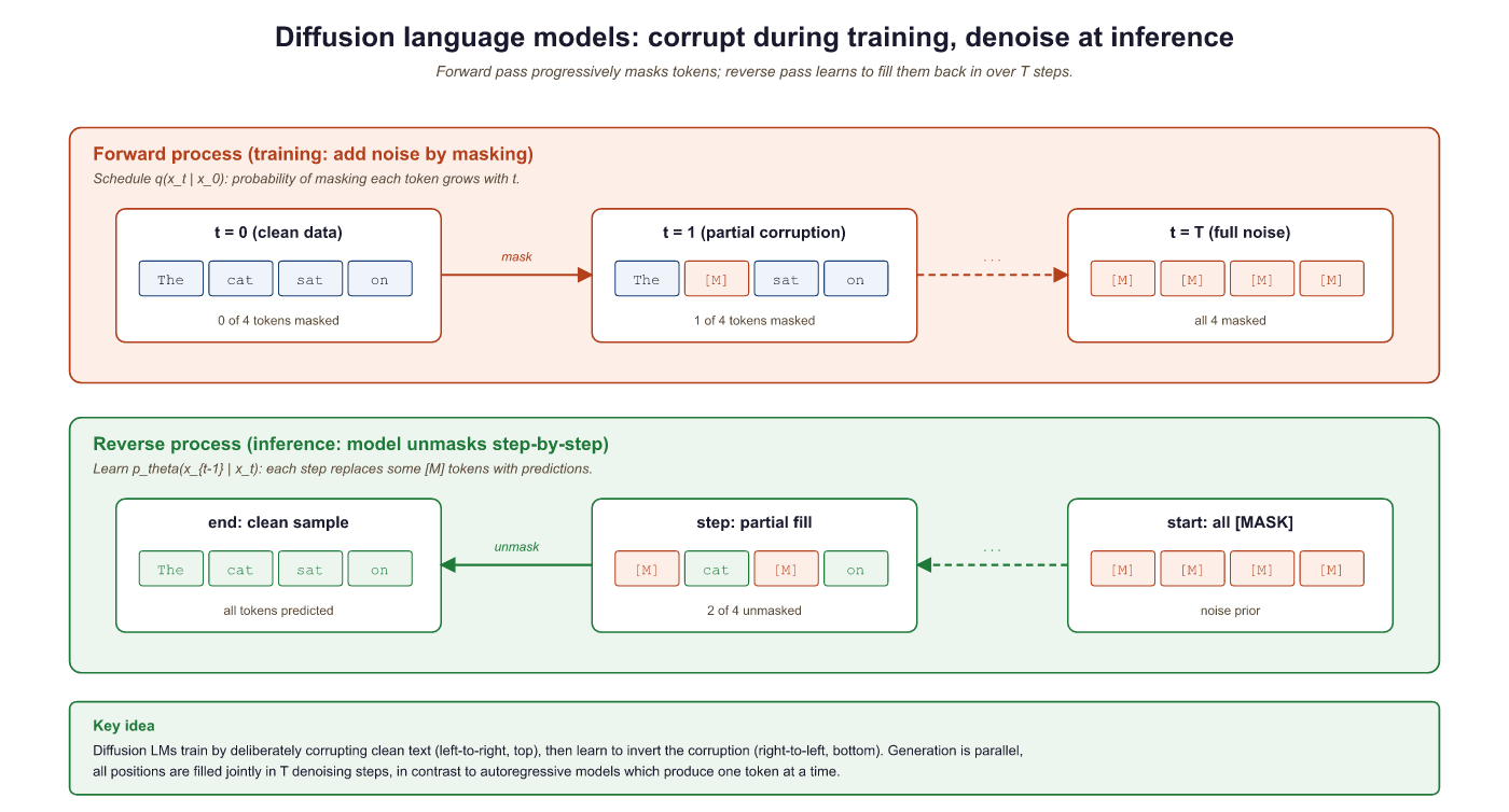
In image diffusion models, the forward process gradually adds Gaussian noise to an image over many steps until it becomes pure noise. The reverse process learns to denoise step by step, recovering the original image. At generation time, you start from random noise and iteratively denoise to produce a new image. This works beautifully because pixel values are continuous, and Gaussian noise is a natural perturbation in continuous space.
Text, however, is discrete: each position holds a token from a finite vocabulary (e.g., 50,000 words). You cannot add Gaussian noise to the word "cat" in any meaningful sense. This fundamental difference requires a completely different formulation of the diffusion process.
The reason diffusion took years to reach language modeling (despite its spectacular success in images) comes down to one word: discreteness. Pixels live in continuous space where you can add a tiny bit of noise and get a slightly blurry image. Tokens live in discrete space where there is no meaningful "halfway" between "cat" and "dog." Replacing Gaussian noise with token masking or substitution was the key conceptual breakthrough that made text diffusion possible.
Who: A research engineering team at a developer tools company investigating faster code completion for their IDE plugin.
Situation: Their existing autoregressive code completion model generated suggestions one token at a time, resulting in noticeable latency (200+ ms) for multi-line completions that frustrated users.
Problem: Users expected near-instant suggestions for common patterns like filling in function bodies or completing boilerplate code, but autoregressive decoding could not generate 50+ tokens fast enough.
Dilemma: Speculative decoding helped but still required sequential verification. Diffusion models offered true parallel generation, but they were less mature for code and harder to control for syntactic correctness.
Decision: The team prototyped a discrete diffusion model (MDLM-based) for infilling tasks, while keeping their autoregressive model for general completions.
How: They trained a discrete absorbing diffusion model on their code corpus, focusing on the infilling task (predicting masked spans within function bodies). They used 10 denoising steps at inference, generating all tokens in parallel at each step.
Result: The diffusion model achieved 3.2x faster generation for infilling tasks of 20 to 80 tokens, with syntactic correctness within 4% of the autoregressive baseline. User satisfaction scores for multi-line completions improved by 18%.
Lesson: Diffusion models excel at tasks where the output length is known and parallel generation matters, but autoregressive models remain superior for open-ended, variable-length generation.
Discrete Diffusion for Text
Instead of adding continuous noise, discrete diffusion corrupts tokens. The most common approach replaces tokens with a special [MASK] token (absorbing diffusion) or with random tokens from the vocabulary (uniform diffusion). Over many forward steps, a clean sentence becomes a sequence of masked or random tokens. The reverse process learns to recover the original tokens from this corrupted state.
Discrete diffusion LMs did not appear from nowhere. The pattern of iteratively re-sampling each token conditioned on the rest is exactly Gibbs sampling, the Markov Chain Monte Carlo (MCMC) algorithm that has been the workhorse of Bayesian latent-variable inference since Geman and Geman (1984). In a Gibbs sweep over a joint distribution $p(z_1, \dots, z_n)$, you fix every coordinate but one, sample $z_i$ from the full conditional $p(z_i \mid z_{-i})$, then move on to $z_{i+1}$; after many sweeps the chain's empirical distribution converges to the target joint. Discrete diffusion's reverse process is the same recipe with two twists. First, the conditionals are no longer derived analytically; they are approximated by a neural network that takes the current (partially masked) sequence and predicts a distribution over each masked token simultaneously. Second, multiple coordinates can be re-sampled per "sweep" rather than one at a time, giving the parallel-generation advantage discussed in Section 4.4.3. The MCMC heritage even rhymes operationally: the 20 to 50 denoising steps modern diffusion LMs use are the analog of MCMC burn-in, and the practical trick of running multiple parallel trajectories (multiple chains) sits inside the same intellectual lineage. Gibbs sampling for Latent Dirichlet Allocation (Blei, Ng, Jordan 2003) is the classic NLP application of the precursor pattern. Readers who want the historical algorithm in detail can consult any textbook on Bayesian methods; deck 0006 in the slide pool gives a self-contained derivation.
4.4.2 Key Models and Approaches
Masked Diffusion Language Model (MDLM) by Sahoo et al. (2024) provides a clean theoretical framework connecting masked language modeling (like Section 7.1) with continuous-time diffusion. The key insight is that BERT-style masked prediction can be viewed as a single-step diffusion process, and extending it to multiple steps with a proper noise schedule yields a full generative model. MDLM achieves competitive perplexity with autoregressive models on standard benchmarks while enabling parallel generation. The discrete-diffusion fundamentals (forward noising, reverse denoising, training objective) appear earlier in Section 4.4.1.
Score Entropy Discrete Diffusion (SEDD) by Lou et al. (2024) introduces a score-based framework for discrete diffusion (see Section 4.4.1 for the underlying noising/denoising loop). Instead of directly predicting denoised tokens, SEDD learns a "score function" that describes how the probability of each token changes as noise is added. This is analogous to score-matching in continuous diffusion and provides a principled training objective. SEDD achieves strong results on text generation and demonstrates the viability of score-based approaches in discrete spaces.
LLaDA (Large Language Diffusion with mAsking, 2025) scales masked diffusion to 8 billion parameters, showing that discrete diffusion models can match autoregressive models in instruction following and reasoning tasks when trained at sufficient scale. Dream (Diffusion Reasoning Model, 2025) extends this with a planner-guided denoising approach that improves coherence for long-form generation. Both models demonstrate that the quality gap between diffusion and autoregressive text generation is closing rapidly.
Cross-Approach Reference Table
Before diving into the individual approaches in the sections that follow, a side-by-side reference anchors the rest of the chapter. The table below summarizes the four families introduced so far, the noise type each uses, the key innovation each contributed, and the failure mode each is best at addressing. Refer back to it whenever the discrete-diffusion taxonomy starts to blur.
| Model | Noise Type | Key Innovation | Scale |
|---|---|---|---|
| MDLM | Absorbing (mask) | Continuous-time diffusion with BERT-like training | Up to 1.1B |
| SEDD | Absorbing (mask) | Score-matching objective for discrete tokens | Up to 1.1B |
| LLaDA | Absorbing (mask) | Scaling to 8B with instruction tuning | 8B |
| Dream | Absorbing (mask) | Planner-guided coherent denoising | 7B |
4.4.3 Parallel Generation: The Speed Advantage
Diffusion models for text generation borrow their core idea from image generation, where you start with pure noise and gradually refine it into a coherent picture. Applying this to language is like sculpting a sentence out of alphabet soup: you start with random letters and iteratively rearrange them until something meaningful emerges.
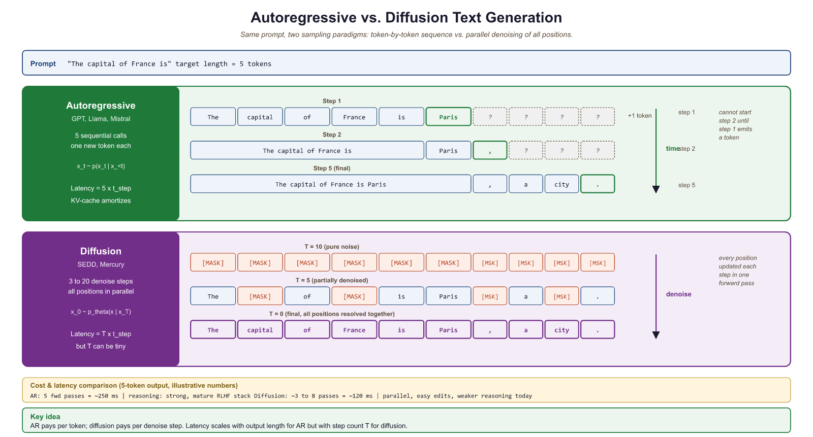
The most exciting property of diffusion language models is parallel token generation. In autoregressive models, generating N tokens requires N sequential forward passes. Each pass depends on the output of the previous one, creating an inherent sequential bottleneck that limits throughput regardless of hardware.
Diffusion models sidestep this entirely. At each denoising step, the model predicts all positions simultaneously. A 1,000-token output might require only 20 to 50 denoising steps, where each step processes the entire sequence in parallel. On modern GPU hardware with massive parallel processing capability, this can translate to order-of-magnitude latency reductions for long outputs.
# Conceptual comparison of generation steps
import numpy as np
def compare_generation_steps(sequence_lengths, diffusion_steps=30):
    """Compare sequential steps needed for AR vs diffusion generation."""
    print(f"{' Length':>8s} | {'AR Steps':>10s} | {'Diffusion Steps':>16s} | {'Speedup':>8s}")
    print("-" * 52)
    for length in sequence_lengths:
        ar_steps = length # one forward pass per token
        diff_steps = diffusion_steps # fixed number of denoising steps
        speedup = ar_steps / diff_steps
        print(f"{length:>8d} | {ar_steps:>10d} | {diff_steps:>16d} | {speedup:>7.1f}x")
compare_generation_steps([50, 200, 500, 1000, 4000])The speedup grows linearly with output length because autoregressive models scale linearly while diffusion models use a fixed number of steps. For a 4,000-token output, the theoretical speedup is over 100x in sequential steps. Of course, each diffusion step processes the entire sequence (which is more expensive per step than a single autoregressive step), so the wall-clock speedup is smaller, typically 3x to 10x for long sequences. Nevertheless, this represents a fundamental architectural advantage.
If the model can predict all positions in one shot, why not run only one denoising step? The reason is the same one classical MCMC practitioners give for burn-in: the first few sweeps of a Markov chain are dominated by the (arbitrary) initialization rather than by the target distribution, and only after many sweeps do samples reflect the true joint. Discrete diffusion inherits this. A single step from a fully masked sequence produces tokens conditioned only on the prompt; subsequent steps then refine each position with the high-confidence skeleton already in place. Empirically, quality climbs rapidly for the first 10 to 20 steps, then plateaus around 30 to 50; pushing past 100 buys little. The autocorrelation problem of MCMC has a faint echo too: drawing intermediate "lag" samples is essentially what confidence-ordered unmasking schedules (used by MDLM, MaskGIT, and Gemini Diffusion) avoid by deliberately spreading the unmasking pattern across the sequence rather than committing to one region at a time. The 20-to-50-step heuristic is therefore not arbitrary; it is the MCMC convergence budget recast for a learned conditional sampler.
# Simplified discrete diffusion process (conceptual)
import torch
def simulate_diffusion_generation(seq_length, vocab_size, num_steps=20):
    """
    Simulate the discrete diffusion generation process.
    At each step, the model predicts all masked positions simultaneously.
    We unmask a fraction of positions per step.
    """
    MASK_TOKEN = vocab_size # special mask token ID
    # Start fully masked
    sequence = torch.full((seq_length,), MASK_TOKEN)
    tokens_per_step = max(1, seq_length // num_steps)
    print(f"Generating {seq_length} tokens in {num_steps} parallel steps\n")
    for step in range(num_steps):
        # Find masked positions
        masked_positions = (sequence == MASK_TOKEN).nonzero(as_tuple=True)[0]
        if len(masked_positions) == 0:
            break
            # "Model prediction": in reality, a neural network predicts all positions
            # Here we simulate by filling with random tokens
            n_to_unmask = min(tokens_per_step, len(masked_positions))
            # Unmask positions with highest "confidence" (simulated)
            chosen = masked_positions[torch.randperm(len(masked_positions))[:n_to_unmask]]
            sequence[chosen] = torch.randint(0, vocab_size, (n_to_unmask,))
            n_remaining = (sequence == MASK_TOKEN).sum().item()
            pct_done = 100 * (1 - n_remaining / seq_length)
            print(f"Step {step+1:2d}: unmasked {n_to_unmask:3d} tokens | {pct_done:5.1f}% complete | {n_remaining:3d} masked")
            return sequence
result = simulate_diffusion_generation(seq_length=100, vocab_size=50000, num_steps=10)# Simplified discrete diffusion for text (conceptual).
# Forward process gradually corrupts tokens; reverse process learns to denoise.
import torch
import torch.nn.functional as F
VOCAB_SIZE = 50257
MASK_TOKEN = VOCAB_SIZE # treat as a sentinel value
def forward_diffusion(tokens: torch.Tensor, t: float) -> torch.Tensor:
"""Forward process: at noise level t in [0,1], replace each token with [MASK]
independently with probability t. At t=1 the entire sequence is masked."""
mask = torch.rand(tokens.shape) < t
return torch.where(mask, torch.full_like(tokens, MASK_TOKEN), tokens)
@torch.no_grad()
def reverse_sample(model, seq_len: int, steps: int = 20) -> torch.Tensor:
"""Reverse process: start from a fully-masked sequence and denoise in `steps`
iterations. At each step the model predicts the original tokens, then we
unmask the ones it's most confident about. After `steps` we have a sample."""
x = torch.full((1, seq_len), MASK_TOKEN, dtype=torch.long)
for step in range(steps):
logits = model(x) # (1, seq_len, vocab+1)
probs = F.softmax(logits, dim=-1)
preds = probs.argmax(dim=-1)
confidence = probs.max(dim=-1).values # (1, seq_len)
# Unmask the K most-confident masked positions
k = max(1, seq_len // steps)
mask_positions = (x == MASK_TOKEN)
scored = confidence * mask_positions
top = scored.topk(k, dim=-1).indices
x.scatter_(1, top, preds.gather(1, top))
return x4.4.4 Gemini Diffusion
Google DeepMind's Gemini Diffusion paradigm applies discrete diffusion at the scale of frontier models (the underlying discrete-diffusion mechanism is covered in Section 4.4.1). While full architectural details remain proprietary, the announced approach combines discrete diffusion with several innovations: adaptive step scheduling (using more denoising steps for complex passages and fewer for simple ones), hierarchical denoising (coarse structure first, fine details later), and integration with the Gemini model family's multimodal capabilities. Early benchmarks suggest latency reductions of 5x to 10x for long-form generation compared to autoregressive Gemini models, with quality approaching (but not yet matching) the autoregressive versions on reasoning-heavy tasks.
The Gemini Diffusion approach, announced in May 2025 at Google I/O, represents the first serious industrial investment in diffusion-based text generation at frontier scale. Google reported a generation speed of roughly 1,479 tokens per second on the experimental release, an order of magnitude faster than autoregressive Gemini 2.0 Flash on comparable hardware. Key reported characteristics include:
- Adaptive denoising schedules: The number of denoising steps is not fixed but varies based on the complexity of what is being generated. Factual recall might need only a few steps, while multi-step reasoning might need dozens. This echoes the adaptive-step-count work in image diffusion (Karras et al., NeurIPS 2022, "Elucidating the Design Space of Diffusion-Based Generative Models"), now ported to text.
- Confidence-ordered unmasking: Tokens the model is most confident about are unmasked first, allowing later steps to condition on the high-confidence "skeleton" of the output. The same idea appeared in MaskGIT (Chang et al., CVPR 2022) for image tokens, and in MDLM (Sahoo et al., NeurIPS 2024) for text; Gemini Diffusion is the first production-scale deployment of the technique.
- Hybrid autoregressive-diffusion: Some implementations use autoregressive generation for the first few tokens (establishing topic and tone) and then switch to diffusion for the bulk of the output. This pattern mirrors the SEDD (Score Entropy Discrete Diffusion, Lou et al., ICML 2024) hybrid decoding mode and is the source of most of the headline latency gains since it amortizes the diffusion-step cost over hundreds of parallel-emitted tokens.
4.4.5 Advantages and Limitations
The Quality Gap for Reasoning
The most significant current limitation of diffusion language models is their performance on tasks requiring complex multi-step reasoning. Autoregressive models naturally "think step by step" because each token is generated in sequence, allowing each step to build on the previous. Diffusion models generate all positions in parallel, which makes it harder to enforce logical dependencies between distant parts of the output. For tasks like mathematical proofs, code generation, and chain-of-thought reasoning, autoregressive models still hold a significant advantage.
The quality gap is not fundamental but practical. Autoregressive models have had years of optimization, scaling, and alignment research (Section 20.1, DPO, constitutional AI). Diffusion language models are still in their early stages. The trajectory of improvement suggests that much of the gap may close as researchers develop diffusion-specific alignment techniques, better noise schedules, and larger-scale training.
4.4.6 TraceRL: Reinforcement Learning for Diffusion LLMs
TraceRL addresses one of the biggest open problems in diffusion language models: how to apply reinforcement learning from human feedback (RLHF) or other reward-based training. In autoregressive models, RLHF is straightforward because each token is a discrete action in a sequential decision process. In diffusion models, the "action" at each step is a parallel update to all positions, making standard RL algorithms inapplicable. TraceRL introduces a "trace-based" reward attribution that propagates reward signals back through the denoising trajectory, enabling effective RL post-training for diffusion language models. Results show significant improvements in instruction following and helpfulness, narrowing the gap with RLHF-trained autoregressive models.
The TraceRL approach works by treating the entire denoising trajectory as a sequence of decisions:
- Generate a complete denoising trajectory: from fully masked to final output, recording the decisions at each step
- Score the final output using a reward model (the same kind used in autoregressive RLHF)
- Attribute the reward back to each denoising step using a credit assignment mechanism inspired by policy gradient methods
- Update the model to increase the probability of denoising trajectories that led to high-reward outputs
This is conceptually similar to how REINFORCE or PPO work in autoregressive models, but adapted for the parallel, iterative structure of diffusion. The "trace" in TraceRL refers to the recorded sequence of denoising steps, which serves as the equivalent of a token-by-token trajectory in autoregressive generation.
# Conceptual pseudocode for TraceRL training loop
# (simplified for illustrative purposes)
def trace_rl_training_step(diffusion_model, reward_model, prompt):
    """One step of TraceRL training (conceptual)."""
    # 1. Generate a denoising trajectory
    trajectory = []
    x_t = initialize_fully_masked(prompt)
    for t in reversed(range(T)):
        # Model predicts which tokens to unmask and what they should be
        predictions, log_probs = diffusion_model.denoise_step(x_t, t)
        trajectory.append({"step": t, "log_probs": log_probs, "state": x_t})
        x_t = apply_predictions(x_t, predictions)
        # 2. Score the final output
        final_text = x_t
        reward = reward_model(prompt, final_text)
        # 3. Compute policy gradient with reward attribution
        loss = 0
        for step_info in trajectory:
            # Attribute reward to each step (with discount)
            step_reward = attribute_reward(reward, step_info["step"], T)
            loss -= step_reward * step_info["log_probs"].mean()
            # 4. Update model
            loss.backward()
            optimizer.step()
            return reward
            # This enables RLHF-style training for diffusion language models,
            # previously an unsolved problem.
            print("TraceRL: enables reward-based training for diffusion LLMs")
print("Key contribution: credit assignment across parallel denoising steps")4.4.7 The Road Ahead
Diffusion-based language models are at a similar stage to where autoregressive transformers were around 2018 to 2019: the fundamental ideas are in place, early results are promising, but enormous scaling and engineering work remains. Several open questions will determine whether diffusion models become a mainstream alternative to autoregressive generation:
- Scaling laws: Do diffusion language models follow similar scaling laws to autoregressive models? Early evidence suggests they do, but with different constants.
- Alignment: Can we develop efficient techniques for aligning diffusion models with human preferences? TraceRL is a first step, but the field needs the equivalent of DPO, constitutional AI, and other alignment breakthroughs.
- Hybrid architectures: Will the future be purely diffusion, purely autoregressive, or a hybrid? Several teams are exploring models that use autoregressive generation for planning and diffusion for execution.
- Multimodal diffusion: Unified diffusion models that generate text, images, code, and structured data simultaneously could be a natural extension of this paradigm.
If this section has piqued your interest, we recommend reading the MDLM and SEDD papers for theoretical foundations, the LLaDA paper for practical scaling, and the TraceRL paper for the alignment frontier. The field is moving fast, and new results appear monthly. Follow the proceedings of NeurIPS, ICML, ICLR, and the ArXiv cs.CL category for the latest developments.
Objective
Implement greedy, top-k, top-p (nucleus), and temperature-scaled decoding from scratch, then compare outputs from a pretrained GPT-2 model using both your manual implementations and the Hugging Face generate() API. You will see how each strategy produces different text characteristics.
Skills Practiced
- Implementing autoregressive decoding with a real language model
- Understanding how temperature, top-k, and top-p shape the output distribution
- Visualizing token probability distributions under different decoding settings
- Comparing manual decoding with Hugging Face's generate() API
Setup
Install the required packages for this lab.
pip install transformers torch matplotlib numpySteps
Step 1: Load a pretrained model and implement greedy decoding
Greedy decoding always picks the highest-probability token. It is deterministic but tends to produce repetitive text. This is the baseline against which all other strategies are compared.
import torch
import numpy as np
from transformers import GPT2LMHeadModel, GPT2Tokenizer
tokenizer = GPT2Tokenizer.from_pretrained("gpt2")
model = GPT2LMHeadModel.from_pretrained("gpt2")
model.eval()
def get_logits(input_ids):
    """Get next-token logits from the model."""
    with torch.no_grad():
        outputs = model(input_ids)
        return outputs.logits[0, -1, :] # logits for the last position
        def greedy_decode(prompt, max_tokens=30):
            """Greedy decoding: always pick the most likely next token."""
            input_ids = tokenizer.encode(prompt, return_tensors="pt")
            generated = list(input_ids[0])
            for _ in range(max_tokens):
                logits = get_logits(torch.tensor([generated]))
                next_token = torch.argmax(logits).item()
                generated.append(next_token)
                if next_token == tokenizer.eos_token_id:
                    break
                    return tokenizer.decode(generated)
                    prompt = "The future of artificial intelligence is"
                    print("GREEDY:")
print(greedy_decode(prompt))Step 2: Implement temperature, top-k, and top-p sampling
Temperature controls the entropy of the sampling distribution (lower = more peaked and deterministic, higher = flatter and more diverse). It does not add "creativity"; it adjusts how uniformly the model samples across its vocabulary. Top-k limits choices to the k most likely tokens. Top-p (nucleus) keeps the smallest set of tokens whose cumulative probability exceeds p.
import torch
def sample_with_strategy(prompt, max_tokens=30, temperature=1.0,
    top_k=0, top_p=1.0):
    """Decode with configurable temperature, top-k, and top-p."""
    input_ids = tokenizer.encode(prompt, return_tensors="pt")
    generated = list(input_ids[0])
    for _ in range(max_tokens):
        logits = get_logits(torch.tensor([generated]))
        # Apply temperature
        logits = logits / temperature
        # Apply top-k filtering
        if top_k > 0:
            top_k_values, _ = torch.topk(logits, top_k)
            threshold = top_k_values[-1]
            logits[logits < threshold] = float("-inf")
            # Apply top-p (nucleus) filtering
            if top_p < 1.0:
                sorted_logits, sorted_indices = torch.sort(logits, descending=True)
                cumulative_probs = torch.cumsum(
                    torch.softmax(sorted_logits, dim=-1), dim=-1)
                # Remove tokens with cumulative probability above the threshold
                sorted_mask = (cumulative_probs
                    - torch.softmax(sorted_logits, dim=-1) >= top_p)
                sorted_logits[sorted_mask] = float("-inf")
                # Scatter back to original indexing
                logits = torch.zeros_like(logits).scatter(
                    0, sorted_indices, sorted_logits)
                # Sample from the filtered distribution
                probs = torch.softmax(logits, dim=-1)
                next_token = torch.multinomial(probs, num_samples=1).item()
                generated.append(next_token)
                if next_token == tokenizer.eos_token_id:
                    break
                return tokenizer.decode(generated)
            prompt = "The future of artificial intelligence is"
            print("TEMPERATURE 0.3 (focused):")
            print(sample_with_strategy(prompt, temperature=0.3))
            print("\nTEMPERATURE 1.5 (creative):")
            print(sample_with_strategy(prompt, temperature=1.5))
            print("\nTOP-K 10:")
            print(sample_with_strategy(prompt, top_k=10))
            print("\nTOP-P 0.9 (nucleus):")
            print(sample_with_strategy(prompt, top_p=0.9))
Step 3: Visualize the probability distributions
Plot how temperature reshapes the token distribution. This makes it concrete why different settings produce different text quality.
import numpy as np
import torch
import matplotlib.pyplot as plt
input_ids = tokenizer.encode(prompt, return_tensors="pt")
logits = get_logits(input_ids)
fig, axes = plt.subplots(1, 3, figsize=(15, 4))
temperatures = [0.3, 1.0, 2.0]
for ax, temp in zip(axes, temperatures):
    probs = torch.softmax(logits / temp, dim=-1).numpy()
    top_indices = np.argsort(probs)[-15:][::-1]
    top_probs = probs[top_indices]
    top_tokens = [tokenizer.decode([i]).strip() for i in top_indices]
    ax.barh(range(len(top_tokens)), top_probs, color="#3498db")
    ax.set_yticks(range(len(top_tokens)))
    ax.set_yticklabels(top_tokens, fontsize=8)
    ax.set_xlabel("Probability")
    ax.set_title(f"Temperature = {temp}")
    ax.invert_yaxis()
    plt.suptitle("How Temperature Reshapes Token Probabilities",
        fontweight="bold")
    plt.tight_layout()
    plt.savefig("decoding_temperature.png", dpi=150)
    plt.show()
Step 4: Compare with Hugging Face generate() API
The library wraps all these strategies (and more) into a single function call. Your from-scratch implementations should produce similar behavioral patterns.
from transformers import set_seed
input_ids = tokenizer.encode(prompt, return_tensors="pt")
set_seed(42)
strategies = {
    "Greedy": dict(max_new_tokens=30, do_sample=False),
    "Top-k (k=10)": dict(max_new_tokens=30, do_sample=True, top_k=10),
    "Top-p (p=0.9)": dict(max_new_tokens=30, do_sample=True, top_p=0.9),
    "Temp 0.3": dict(max_new_tokens=30, do_sample=True, temperature=0.3),
    "Beam (n=4)": dict(max_new_tokens=30, num_beams=4, do_sample=False),
    }
print(f"Prompt: '{prompt}'\n")
for name, kwargs in strategies.items():
    set_seed(42)
    output = model.generate(input_ids, **kwargs,
        pad_token_id=tokenizer.eos_token_id)
    text = tokenizer.decode(output[0], skip_special_tokens=True)
    print(f"{name:15s}: {text}")
    print("\nFrom scratch: ~60 lines per strategy.")
print("Hugging Face: 1 line per strategy with generate().")Stretch Goals
- Implement beam search from scratch and compare its output with Hugging Face's beam search on the same prompt.
- Add repetition penalty to your sampler (divide logits of already-generated tokens by a penalty factor) and observe how it reduces loops.
- Run each strategy 10 times on the same prompt and measure diversity (unique n-grams) vs. coherence (perplexity) to quantify the exploration and exploitation tradeoff.
- Discrete diffusion adapts the diffusion framework from images to text by replacing continuous Gaussian noise with token masking or random replacement.
- Key models (MDLM, SEDD, LLaDA, Dream) have demonstrated that diffusion language models can achieve competitive quality with autoregressive models, especially at scale.
- The primary advantage is parallel generation: all tokens are produced simultaneously across a fixed number of denoising steps, providing order-of-magnitude latency reduction for long outputs.
- Gemini Diffusion represents the first frontier-scale industrial deployment of diffusion-based text generation, with adaptive step scheduling and hybrid approaches.
- The primary limitation is a quality gap on reasoning tasks, where the sequential nature of autoregressive generation provides a natural advantage for chain-of-thought style computation.
- TraceRL (ICLR 2026) opens the door to RLHF-style alignment for diffusion models by solving the credit assignment problem across parallel denoising steps.
- The field is evolving rapidly. Hybrid autoregressive-diffusion architectures and diffusion-specific alignment techniques are active areas of research.
Show Answer
Show Answer
Show Answer
Show Answer
Exercises
An autoregressive model takes 50ms per token. A diffusion model takes 200ms per denoising step and uses 30 steps regardless of output length (parallel generation across all positions). Compute the wall-clock latency for outputs of length (a) 50 tokens, (b) 200 tokens, (c) 1000 tokens. (d) At what output length do the two approaches break even?
Answer Sketch
(a) AR: 50 × 50ms = 2.5s. Diffusion: 30 × 200ms = 6s. AR is 2.4x faster for short outputs. (b) AR: 200 × 50ms = 10s. Diffusion: 6s. Diffusion is now 1.67x faster. (c) AR: 1000 × 50ms = 50s. Diffusion: still 6s. Diffusion is 8.3x faster. (d) Break-even: 50ms × N = 30 × 200ms, so N = 6000/50 = 120 tokens. Below 120 tokens, AR wins; above, diffusion wins. The crossover scales with: (denoising_steps × per_step_time) / per_token_AR_time. Optimization knobs: reducing diffusion steps (Gemini Diffusion uses adaptive step counts down to 8-15) lowers the crossover; faster AR per-token (KV caching, FlashAttention) raises it. The economic implication: diffusion is preferred for streaming applications where 1000+ token outputs are common, while AR remains preferred for short Q&A.
Image diffusion adds Gaussian noise to continuous pixel values. Text tokens are discrete. (a) Explain why "add Gaussian noise to token IDs" fails as an analog. (b) Compare two discrete diffusion approaches: absorbing (mask-based) vs. uniform (random-replacement). (c) Predict which would learn faster on text and why.
Answer Sketch
(a) Token IDs are arbitrary integers with no semantic ordering: ID 1234 ("the") and ID 1235 ("them") may be very different words. Adding Gaussian noise (e.g., 1234 + 0.5) produces non-integer values that don't correspond to any token, or rounds to neighboring IDs that have no semantic relationship. The noise model must respect the discrete vocabulary structure. (b) Absorbing diffusion: at each forward step, replace tokens with [MASK] with growing probability; at the end, all tokens are [MASK]. The reverse process learns to fill in masked tokens. Uniform diffusion: at each forward step, replace tokens with a random vocabulary token with growing probability; at the end, all tokens are uniform random. (c) Absorbing typically learns faster because [MASK] is a clear "I don't know" signal that the model interprets unambiguously, similar to BERT's MLM task that the model already excels at. Uniform corruption requires the model to figure out which tokens are real vs noise, a harder discrimination task. Empirically, MDLM (absorbing) outperforms SEDD-uniform at equal compute.
Diffusion language models sometimes produce outputs where individual sentences are fluent but the overall narrative is incoherent. (a) Why does parallel generation make this failure mode more likely? (b) Sketch a concrete example. (c) Describe one mitigation that hybrid autoregressive-diffusion models use to address this.
Answer Sketch
(a) In autoregressive generation, every token is conditioned on all previous tokens, so the model can reference "the dog Spot from sentence 1" when writing sentence 5. In diffusion, all tokens are generated in parallel from a noisy initial state, refined over a fixed number of denoising steps. There is no natural mechanism for token at position 200 to "wait for" token at position 50 to settle before being decided. Each denoising step updates all positions simultaneously, so coordination across long distances must emerge from the iterative refinement, not from explicit causal dependence. (b) Example: prompt "Write a short story about a detective named Sara investigating a missing painting." Diffusion output: paragraph 1 introduces "Detective Sara"; paragraph 2 talks about "the painting case"; paragraph 3 suddenly refers to "Inspector John" and "the missing necklace" because positions in paragraph 3 settled on different name/object decisions than positions in paragraph 1. (c) Hybrid mitigation: Generate the first 100 tokens autoregressively (establishing entities, plot points), then use diffusion to fill in the remainder conditioned on the autoregressive prefix as fixed context. This combines AR's coherence-establishing strengths with diffusion's parallel-generation speed. Variants: AR generates "key" tokens (named entities, structural markers), diffusion fills the connective tissue.
You have a diffusion LM that uses 50 denoising steps by default. (a) If you reduce to 25 steps with no other changes, predict the impact on (i) latency, (ii) quality, (iii) variance across runs. (b) What advanced technique would let you maintain quality at 10 steps?
Answer Sketch
(a)(i) Latency halves linearly: 50 → 25 steps cuts wall-clock by 2x. (ii) Quality degrades because each step does less denoising work; the per-step "denoising budget" is now larger, so the model takes bigger jumps and may miss the high-density regions of the output distribution. Empirical degradation: ~10-30% on standard benchmarks for going 50→25, more for going 50→10. (iii) Variance increases: with fewer refinement steps, the model has less opportunity to correct mistakes, so the final output is more sensitive to the initial noise sample. Multiple runs of the same prompt produce more divergent outputs. (b) Advanced techniques: (i) Distillation: train a "few-step" student model to mimic the multi-step teacher's output, similar to progressive distillation in image diffusion (DDIM → consistency models). (ii) Adaptive step scheduling: spend more steps in the high-uncertainty middle of the denoising trajectory and fewer at the extremes. Gemini Diffusion uses adaptive scheduling to achieve good quality at 8-15 steps. (iii) Speculative diffusion: use a fast small model to propose updates that the larger model verifies, analogous to speculative decoding for AR.
RLHF for autoregressive models treats each generated token as a discrete "action" in a sequential MDP. TraceRL adapts RLHF to diffusion. (a) Why doesn't the standard MDP formulation directly work for diffusion? (b) What does TraceRL use as the analog of an "action"? (c) What does this enable that wasn't possible before?
Answer Sketch
(a) In standard MDP RLHF: state = prefix of tokens generated so far; action = next token; trajectory = sequence of (state, action) pairs; reward at end gets credit-assigned via PPO using each action's log-probability. For diffusion: there is no "next token"; each denoising step updates all positions simultaneously. The "trajectory" is a sequence of denoising steps where each step produces an entire sequence (the partial denoised output). Standard PPO formulas don't apply because actions are not discrete tokens but continuous distributions over many positions. (b) TraceRL treats each denoising step as an action, where the action is the change made to the noisy sequence at that step. The trajectory is the sequence of denoising steps from pure noise to final output. The reward at the end is credit-assigned across denoising steps using a "trace" of how each step contributed to the final output (computed via gradient attribution or by replaying the trajectory under different perturbations). (c) This enables RLHF-style preference optimization for diffusion LMs, allowing them to be aligned to human preferences just like AR models. Before TraceRL, diffusion LMs could only be supervised-fine-tuned, missing the safety/quality alignment that RLHF provides for AR models. TraceRL is the first technique that fully closes this alignment gap.
For each scenario, predict whether AR or diffusion would be better, and why. (a) A chatbot answering 1-2 sentence questions. (b) A code generation tool that produces 500-line files. (c) A document-rewriting tool that needs to make many small edits to a 10,000-token document. (d) Step-by-step math solving (chain-of-thought).
Answer Sketch
(a) AR. Short outputs (under ~120 tokens given typical break-evens) favor AR's lower fixed cost. Also, chat is interactive and benefits from streaming, which AR provides naturally. (b) Tossup, leaning diffusion for raw speed but AR for code quality. Code requires precise long-range structural coherence (matching brackets, consistent variable names) that diffusion currently struggles with. The latency win of diffusion is significant for 500 lines, but quality may not yet be acceptable for production code. As of 2026, AR with KV caching is still preferred for code; this may shift as diffusion code models mature. (c) Diffusion. Document editing is exactly where diffusion shines: starting from "noisy" (current) text and iteratively refining toward a target. Inserting/deleting tokens at multiple locations in parallel is the natural diffusion operation. AR would need to regenerate large spans even for small edits. Tools like Gemini Diffusion are positioning specifically for this use case. (d) AR. Chain-of-Thought is the canonical case where sequential dependence between tokens matters. Each step depends on all previous reasoning. Diffusion's parallel generation directly conflicts with the sequential nature of CoT. Until hybrid approaches mature, AR remains the only choice for serious reasoning workloads.
Congratulations: you have completed Part I. You now understand the full pipeline from raw text to generated output: NLP fundamentals and tokenization basics (Chapter 1), embeddings (Chapter 1), sequence modeling (Chapter 2), the Transformer architecture (Chapter 3), and decoding algorithms (Chapter 05). In Part II: Understanding LLMs, you will see how these foundations scale. Chapter 6 covers pretraining and scaling laws: how models like GPT-3 are trained on trillions of tokens and why larger models exhibit emergent capabilities. Chapter 7 dives deeper into tokenization, and Chapter 9 covers alignment and RLHF. Together, Parts I and II give you the complete picture needed for the applied chapters in Parts III and IV.
Discrete diffusion is evolving rapidly (the foundational forward-noising and reverse-denoising loop is unpacked in Section 4.4.1). Mercury (Inception Labs, 2025) achieved the first production-quality diffusion LLM, generating 1,000+ tokens per second by producing multiple tokens simultaneously. MDLM (Sahoo et al., 2024) and SEDD (Lou et al., 2024) established competitive benchmarks for discrete diffusion language modeling. However, autoregressive models still dominate in practice due to their superior instruction-following ability and the mature infrastructure surrounding them.
Always set max_tokens (or max_new_tokens) in production. Without it, a model can generate indefinitely, burning through your API budget or GPU memory. Start conservative (256 tokens for short tasks) and increase based on observed needs.
What's Next?
In the next chapter, Chapter 6: Pretraining, Scaling Laws & Data Curation, we begin Part II by examining how LLMs are pretrained at scale, including scaling laws and data curation strategies.