Alternative Architectures Beyond Transformers

"The transformer is not the end of history. It is the beginning of the search for something better."

Frontier, Architecture Restless AI Agent

75.3.1 The Scaling Problem with Self-Attention

What if your electricity bill doubled every time you tried to read a longer document? That is essentially the economics of standard self-attention. It computes a pairwise similarity score between every token in a sequence and every other token. For a sequence of length n, this produces an n x n attention matrix, requiring $O(n^{2})$ time and memory. At a sequence length of 2,048 tokens, the attention matrix contains roughly 4 million entries. At 128K tokens, it balloons to over 16 billion entries. Even with FlashAttention and other optimizations (covered in Section 9.1), the fundamental quadratic relationship remains.

This bottleneck manifests in three practical ways. First, training cost: doubling the context window roughly quadruples the compute required for the attention layers. Second, inference latency: the KV cache grows linearly with sequence length, consuming GPU memory and slowing each decoding step. Third, accessibility: long-context transformer inference requires high-end GPUs, putting it out of reach for edge devices, embedded systems, and cost-sensitive deployments.

The alternative architectures surveyed in this section all attack this quadratic bottleneck, but they use different strategies and accept different tradeoffs. Some replace attention entirely. Others retain attention in a limited capacity and pair it with more efficient mechanisms. Understanding these tradeoffs is essential for choosing the right architecture for a given deployment scenario.

75.3.2 State Space Models: S4, Mamba, and Mamba-2

State space models (SSMs) originated in control theory, where they describe systems that maintain a hidden state vector and update it at each timestep based on the current input. The key insight is that the hidden state has a fixed size regardless of how many timesteps have elapsed, giving SSMs $O(n)$ time complexity for sequences of length n.

Side-by-side, a transformer block runs the token sequence through self-attention with $O(n^2)$ compute and a growing KV cache, then a feed-forward network. A Mamba block instead runs the sequence through input-dependent A, B, C, dt selection followed by a parallel scan with $O(n)$ compute and a fixed-size hidden state, then a feed-forward network. The trade-off is explicit: Mamba wins on linear scaling and streaming inference, while transformers retain full content access through their attention pattern.

75.3.2.1 The S4 Foundation

The Structured State Space for Sequence Modeling (S4) paper by Gu et al. (2022) demonstrated that parameterizing state space models with specific matrix structures could make them competitive with transformers on long-range benchmarks. S4 models the sequence-to-sequence mapping as a continuous-time system discretized for digital processing:

# S4 state space model (simplified)
# Continuous-time formulation:
# x'(t) = A x(t) + B u(t) (state evolution)
# y(t) = C x(t) + D u(t) (output)
#
# Discretized for step size delta:
# x_k = A_bar x_{k-1} + B_bar u_k
# y_k = C x_k + D u_k
import torch
import torch.nn as nn
class SimpleSSMLayer(nn.Module):
    """Simplified state space model layer for illustration."""
def __init__(self, d_model: int, state_dim: int = 64):
    super().__init__()
    self.d_model = d_model
    self.state_dim = state_dim
    # Learnable state space parameters
    self.A = nn.Parameter(torch.randn(state_dim, state_dim) * 0.01)
    self.B = nn.Parameter(torch.randn(state_dim, d_model) * 0.01)
    self.C = nn.Parameter(torch.randn(d_model, state_dim) * 0.01)
    self.D = nn.Parameter(torch.ones(d_model)) # skip connection
    # Discretization step size
    self.log_delta = nn.Parameter(torch.zeros(d_model))
def forward(self, u: torch.Tensor) -> torch.Tensor:
    """
    Process sequence with linear recurrence.
    u: (batch, seq_len, d_model)
    returns: (batch, seq_len, d_model)
    """
    batch, seq_len, _ = u.shape
    delta = torch.exp(self.log_delta)
    # Discretize continuous parameters (simplified Euler method)
    A_bar = torch.eye(self.state_dim, device=u.device) + delta.mean() * self.A
    B_bar = delta.mean() * self.B
    # Recurrent scan through sequence
    x = torch.zeros(batch, self.state_dim, device=u.device)
    outputs = []
    for k in range(seq_len):
        x = A_bar @ x.unsqueeze(-1) + (B_bar @ u[:, k].unsqueeze(-1))
        x = x.squeeze(-1)
        y_k = (self.C @ x.unsqueeze(-1)).squeeze(-1) + self.D * u[:, k]
        outputs.append(y_k)
        return torch.stack(outputs, dim=1)

Code 34.3.1: Simplified state space model layer showing the recurrence pattern. Production implementations use parallel scan algorithms for GPU efficiency rather than sequential loops.

The critical property of S4 is that the recurrence x_k = A_bar * x_{k-1} + B_bar * u_k can be computed in two modes. During training, the recurrence can be unrolled into a convolution, enabling parallel computation across the entire sequence on a GPU. During inference, the model operates as a true recurrence: it updates the state with each new token and produces output in $O(1)$ per step, with no KV cache that grows with sequence length. This dual mode is a fundamental advantage over transformers.

75.3.2.2 Mamba: Selective State Spaces

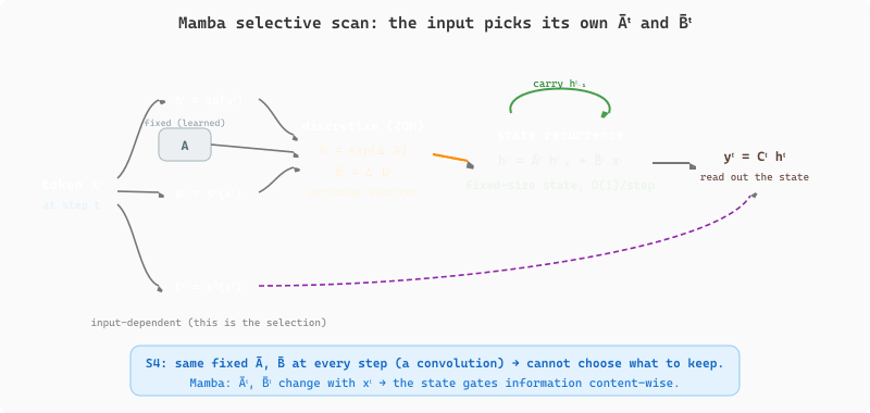
Mamba (Gu and Dao, 2023) addressed a key limitation of S4: the state transition matrices A and B were fixed for all inputs, meaning the model could not dynamically decide what information to retain or discard based on the current token. Mamba introduced selective scan, where B, C, and the discretization step delta are computed as functions of the input at each timestep.

Figure 75.3.2 shows the mechanism: each token $x_t$ produces its own $\Delta_t$, $B_t$, and $C_t$, which discretize $A$ and $B$ into the input-dependent $\bar{A}_t$ and $\bar{B}_t$ that gate the state recurrence, so the same hidden state can be made to remember or forget depending on what arrives.

from torch import nn
import torch
# Mamba selective scan (conceptual)
# Key difference from S4: B, C, and delta are input-dependent
class SelectiveSSM(nn.Module):
    """Mamba-style selective state space model (simplified)."""
    def __init__(self, d_model: int, state_dim: int = 16, expand: int = 2):
        super().__init__()
        d_inner = d_model * expand
        # Input projection (expand dimension)
        self.in_proj = nn.Linear(d_model, d_inner * 2, bias=False)
        # Input-dependent parameter projections
        self.B_proj = nn.Linear(d_inner, state_dim, bias=False)
        self.C_proj = nn.Linear(d_inner, state_dim, bias=False)
        self.delta_proj = nn.Linear(d_inner, d_inner, bias=True)
        # Fixed A (diagonal, initialized with log-spaced values)
        A = torch.arange(1, state_dim + 1, dtype=torch.float32)
        self.log_A = nn.Parameter(torch.log(A).unsqueeze(0).expand(d_inner, -1))
        # Output projection
        self.out_proj = nn.Linear(d_inner, d_model, bias=False)
    def forward(self, x: torch.Tensor) -> torch.Tensor:
        """
        x: (batch, seq_len, d_model)
        """
        batch, seq_len, _ = x.shape
        # Project and split into two paths
        xz = self.in_proj(x)
        x_path, z_path = xz.chunk(2, dim=-1)
        # Compute input-dependent parameters
        B = self.B_proj(x_path) # (batch, seq, state_dim)
        C = self.C_proj(x_path) # (batch, seq, state_dim)
        delta = torch.softplus( # (batch, seq, d_inner)
            self.delta_proj(x_path)
            )
        A = -torch.exp(self.log_A) # (d_inner, state_dim)
        # Selective scan (in practice, uses custom CUDA kernel)
        y = self._selective_scan(x_path, A, B, C, delta)
        # Gated output
        y = y * torch.silu(z_path)
        return self.out_proj(y)
    def _selective_scan(self, u, A, B, C, delta):
        """Hardware-aware selective scan (simplified)."""
        batch, seq_len, d_inner = u.shape
        state_dim = A.shape[-1]
        # In production: parallel associative scan on GPU
        # Here: sequential for clarity
        h = torch.zeros(batch, d_inner, state_dim, device=u.device)
        outputs = []
        for t in range(seq_len):
            # State update with input-dependent gating
            A_t = torch.exp(delta[:, t, :, None] * A[None, :, :])
            B_t = delta[:, t, :, None] * B[:, t, None, :]
            h = A_t * h + B_t * u[:, t, :, None]
            y_t = (h * C[:, t, None, :]).sum(dim=-1)
            outputs.append(y_t)
            return torch.stack(outputs, dim=1)

Code 34.3.2: Simplified Mamba selective scan. The input-dependent B, C, and delta projections are the key innovation: the model learns what to remember and what to forget at each step.

# Production Mamba using the official package
from mamba_ssm import Mamba
model = Mamba(
    d_model=512,
    d_state=16,
    d_conv=4,
    expand=2,
    ).cuda()
y = model(x) # Uses hardware-optimized parallel scan

Input: sequence u = [u1, ..., uL], model parameters (A, B_proj, C_proj, Δ_proj)
Output: output sequence y = [y1, ..., yL]
1. Initialize hidden state h = 0
2. for t = 1 to L:
3. // Input-dependent parameter computation
a. Bt = B_proj(ut) // project input to get B
b. Ct = C_proj(ut) // project input to get C
c. Δt = softplus(Δ_proj(ut)) // input-dependent step size
4. // Discretize and update state
d. Āt = exp(Δt · A) // discretized transition
e. B̄t = Δt · Bt // discretized input
f. h = Āt ⊙ h + B̄t ⊙ ut // state update (element-wise)
g. yt = Ct · h // output from state
5. return y

The selectivity mechanism makes Mamba data-dependent: it can choose to "open the gate" for important tokens (like a keyword in a retrieval task) and "close the gate" for irrelevant ones (like filler words). This is conceptually similar to how attention selectively focuses on relevant tokens, but it operates through a compressed state vector rather than explicit pairwise comparisons.

75.3.2.3 Mamba-2: Structured State Space Duality

Mamba-2 (Dao and Gu, 2024) revealed a deep mathematical connection: the selective scan operation in Mamba is equivalent to a form of structured linear attention when viewed through the right lens. This "state space duality" (SSD) framework unifies SSMs and attention under a single theoretical umbrella, showing that they are two computational paths for the same underlying operation.

Practically, Mamba-2 achieves 2-8x speedups over Mamba-1 by exploiting this duality. The SSD layer uses a block-decomposition that processes chunks of the sequence using efficient matrix multiplications (the "attention-like" view) while maintaining the recurrent state across chunks (the "SSM view"). This means Mamba-2 gets the best of both worlds: the parallelism of attention during training and the constant-memory inference of recurrence during generation.

By 2026 the pure-SSM lineage has largely given way to hybrid SSM-transformer production models that interleave a few full-attention layers among many SSM layers, recovering the long-range recall that pure SSMs sacrifice. The reference open-weight hybrids are Jamba (AI21, 2024, a Mamba-Transformer-MoE), Zamba (Zyphra, 2024), and Falcon-H1 (TII, 2025); on the linear-recurrent side, xLSTM (Beck et al., 2024) revives the LSTM with exponential gating and matrix memory. The recurring lesson is that a small fraction of attention layers is enough to close most of the quality gap while keeping most of the inference-time memory savings.