"We keep scaling until the electricity bill becomes the research contribution."
Frontier, Budget Busting AI Agent
The era of "just scale up the Transformer architecture on more internet text" is approaching its limits. The next generation of frontier models will be shaped by constraints: finite high-quality data, the economics of compute, and the diminishing returns of naive scaling. This section maps the three axes along which scaling can proceed (data, compute, test-time inference) and surveys the architectural alternatives that may reshape the landscape. Understanding these frontiers is essential for anyone making multi-year bets on AI infrastructure, model selection, or research direction.
Prerequisites
This section builds on pretraining data and scaling laws from Chapter 6, inference optimization from Chapter 9, and synthetic data generation from Chapter 15. Familiarity with the Chinchilla scaling laws (Section 6.3) is especially important.
75.2.1 The Data Wall
The Chinchilla scaling laws (Hoffmann et al., 2022), covered in Section 6.3, established that optimal training requires scaling data and compute proportionally. For a model with N parameters, you need roughly 20N tokens of training data to achieve compute-optimal performance. This creates a straightforward problem: where do those tokens come from?
How Much Data Exists?
Villalobos et al. (2024) at Epoch AI conducted the most systematic analysis of this question. Their estimates suggest that the total stock of publicly available, high-quality text on the internet is between 4 and 15 trillion tokens, depending on quality thresholds. Lower-quality text (scraped web pages without filtering) extends this to perhaps 30 to 50 trillion tokens, but with rapidly diminishing quality.
To put this in perspective: GPT-4 is estimated to have been trained on approximately 13 trillion tokens (OpenAI has not disclosed GPT-4's size or token count; these figures come from industry reporting and are unconfirmed). Llama-3 (405B) was trained on 15 trillion tokens. If the Chinchilla-optimal data requirement for a 10-trillion-parameter model is 200 trillion tokens, we have a problem. The internet does not contain enough high-quality text to support the next order-of-magnitude increase in model size.
The data wall is not just about volume. It is also about diversity. As models absorb more of the available text, each additional token provides less novel information. The marginal value of the 15-trillionth token is far less than the marginal value of the 1-trillionth token, because it is increasingly likely to be a paraphrase of content already seen.
Responses to the Data Wall
Frontier labs are pursuing several strategies simultaneously:
- Multi-epoch training. Training on the same data multiple times. Early evidence suggested this was harmful, but recent work shows that with proper learning rate scheduling and data ordering, models can extract additional value from repeated passes (Muennighoff et al., 2023). The penalty for repetition is real but manageable for 2 to 4 epochs.
- Data curation and filtering. Rather than gathering more data, improve the quality of existing data. Techniques include perplexity filtering, deduplication, classifier-based quality scoring, and domain rebalancing. The FineWeb dataset (Penedo et al., 2024) demonstrated that aggressive quality filtering of Common Crawl can produce training data that matches or exceeds curated datasets at a fraction of the size.
- Synthetic data generation. Using existing models to generate training data for the next generation. This is covered in detail in Chapter 15, but the frontier implications deserve attention here.
- Multimodal data. Supplementing text with images, video, audio, and code. A single YouTube video contains both visual and auditory information that, when transcribed and aligned, provides a richer learning signal than text alone.
- Private and licensed data. Partnerships with publishers, news organizations, and data aggregators. These deals (e.g., OpenAI's agreements with the Associated Press and News Corp) are partly about data access and partly about legal risk mitigation.
Humanity spent thousands of years producing the written record. Frontier labs consumed most of it in a single training run. The internet, it turns out, is a surprisingly finite resource when your appetite is measured in trillions of tokens.
75.2.2 Synthetic Data: Promise and Peril
The most controversial response to the data wall is synthetic data: using model-generated text to train the next generation of models. The promise is obvious. If a frontier model can generate high-quality text, that text can be used to train a larger model, creating a virtuous cycle that decouples scaling from the finite stock of human-generated data.
Where Synthetic Data Works
Synthetic data has proven effective in specific, constrained domains:
- Mathematics and code. Models can generate vast quantities of mathematical proofs and programming problems with verifiable solutions. The verification step (can the proof be checked? does the code pass tests?) provides a natural quality filter. This is the strategy behind approaches like AlphaProof and the mathematical reasoning improvements in recent models.
- Instruction tuning. The Evol-Instruct approach (Xu et al., 2023), covered in Section 15.2, generates increasingly complex instruction-response pairs by iteratively rewriting prompts. This has been widely adopted, with WizardLM and its successors demonstrating that synthetic instruction data can match or exceed human-written instructions for fine-tuning.
- Distillation. Using a larger model's outputs to train a smaller model, as covered in Chapter 17. This is technically synthetic data, and it works well because the teacher model provides a richer training signal (soft probabilities) than the original hard labels.
Model Collapse: The Danger
Shumailov et al. (2024), published in Nature, demonstrated a sobering phenomenon they termed "model collapse." When models are trained on data generated by previous model generations, the distribution of the training data narrows progressively. Rare events, tail phenomena, and minority perspectives are gradually lost. After several generations of recursive training, the model's output distribution converges to a narrow mode that no longer reflects the diversity of the original human-generated data.
The analogy is photocopying a photocopy: each generation loses fidelity, and the losses compound. The authors showed this effect across multiple model families and training setups, suggesting it is a fundamental property of iterative synthetic data generation rather than an artifact of a particular approach.
The practical implication is that synthetic data can supplement human data but probably cannot fully replace it. A training pipeline that relies primarily on synthetic data will need robust mechanisms to detect and counteract distribution narrowing, such as diversity metrics, tail-event preservation, and periodic infusion of human-generated data.
Synthetic data is like maintaining a sourdough starter. You can refresh it indefinitely by feeding it flour (compute), and the active cultures (knowledge) persist across generations. But if you only ever feed it the same flour, the microbial diversity narrows. Occasionally, you need to introduce wild yeast (human-generated data) from a new source to maintain a healthy, diverse culture. A purely self-referential starter eventually produces bland, uniform bread.
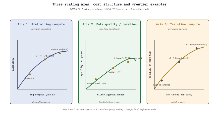
75.2.3 The Three Axes of Scaling
Historically, scaling meant one thing: bigger pretraining runs (more parameters, more data, more compute). But the frontier has diversified into three distinct scaling axes, each with different economics and different diminishing returns profiles.
Axis 1: Pretraining Compute
This is the traditional scaling axis. Train a larger model on more data. The cost grows roughly quadratically with model size (because both the number of parameters and the data requirement increase). Frontier training runs in 2025 are estimated to cost $100 million to $1 billion. The returns, as measured by benchmark improvements, are diminishing: each doubling of compute yields smaller absolute gains.
Axis 2: Data Quality and Curation
The Llama strategy (Touvron et al., 2023) demonstrated an alternative: train a smaller model for longer on higher-quality data. Llama 1 (65B) was trained on 1.4 trillion tokens, far exceeding the Chinchilla-optimal data allocation for its size. This "over-training" approach produces models that are less compute-efficient during training but more token-efficient during inference, because the resulting model is smaller and cheaper to serve.
This insight has reshaped the industry. Most practitioners serve models, not train them. A model that costs twice as much to train but is half the size at serving time is often the better economic choice. The data quality axis offers a way to improve performance without increasing model size, by investing in better data curation, filtering, and curriculum design.
Axis 3: Test-Time Compute
The most significant recent development is the emergence of test-time compute scaling, as discussed in the context of reasoning models in Section 7.4. Models like OpenAI's o1 and o3, DeepSeek-R1, and Anthropic's extended thinking demonstrate that spending more compute at inference time (through chain-of-thought reasoning, search, verification, and self-correction) can dramatically improve performance on hard tasks.
The economics of test-time scaling are fundamentally different from pretraining scaling. Pretraining is a one-time cost amortized over all future queries. Test-time compute is a per-query cost that scales linearly with usage. This means test-time scaling is most cost-effective for hard, high-value queries where the additional compute is justified by the value of a correct answer.
The interplay between pretraining and test-time compute creates interesting trade-offs. A smaller, well-trained model with generous test-time compute can sometimes match a much larger model with minimal test-time compute. The optimal allocation depends on the query distribution: if most queries are easy, invest in pretraining; if a few queries are very hard and high-value, invest in test-time compute.
Reasoning models bill you per thought. An o3 high-reasoning answer might consume 20,000 hidden chain-of-thought tokens to produce a 200-token reply, and you pay for all 20,200. The economic model has quietly shifted from "buy the right model for the job" to "buy the right amount of thinking for the job", which means a frontier API call's price tag now varies more by reasoning budget than by which provider you picked. Several teams discovered this when their monthly bill tripled the day they flipped reasoning_effort: high as a default.
The table below summarizes how these three scaling axes differ in their cost structure, return profiles, and ideal use cases.
| Scaling Axis | Cost Structure | Diminishing Returns | Best For |
|---|---|---|---|
| Pretraining compute | One-time, amortized | Moderate (power law) | General capability uplift |
| Data quality | One-time curation investment | Low (quality improvements compound) | Efficiency, smaller serving models |
| Test-time compute | Per-query, variable | Task-dependent | Hard tasks, high-value queries |
Notice that pretraining compute and data quality are one-time investments, while test-time compute is an ongoing per-query expense. This asymmetry is central to the economic calculus of frontier model development.
The three scaling axes are not independent; they interact. A model trained on better data (Axis 2) may need less test-time compute (Axis 3) because it has stronger priors. A model with more pretraining compute (Axis 1) may benefit less from test-time reasoning because it has already internalized the relevant knowledge. The optimal scaling strategy for a given application depends on the query mix, the cost constraints, and the latency requirements. There is no universally optimal allocation. The practical implication for teams making deployment decisions (see the cost analysis in Section 31.8) is to benchmark each axis independently for your specific use case rather than relying on general-purpose scaling curves.
75.2.4 Alternative Architectures
Beyond scaling existing transformers along these three axes, a separate question looms: is the transformer itself the right architecture? The transformer has dominated language modeling since 2017, but several alternative architectures are challenging its supremacy, particularly for long-context and efficiency-critical applications.
State Space Models (SSMs)
State space models, particularly the Mamba architecture (Gu and Dao, 2023), offer a fundamentally different approach to sequence modeling. Instead of the quadratic attention mechanism, SSMs process sequences through a linear recurrence that scales linearly with sequence length. This makes them dramatically more efficient for long sequences.
The key insight behind Mamba is the "selective state space" mechanism, which allows the model to selectively propagate or forget information based on the input content. This addresses the principal limitation of earlier SSMs, which processed all tokens identically regardless of content relevance.
As of early 2026, SSMs have demonstrated competitive performance with transformers on many benchmarks, with clear advantages in throughput for long sequences. However, they have not yet matched transformers on tasks that require complex in-context learning or precise information retrieval from context. Hybrid architectures that combine transformer attention layers with SSM layers are emerging as a pragmatic compromise, offering the efficiency of SSMs for most processing while retaining attention for tasks that require it.
Mamba inherits the continuous form of a linear time-invariant state space model: $\dot{h}(t) = A\, h(t) + B\, u(t)$ with output $y(t) = C\, h(t)$. For discrete tokens, the recurrence is obtained through zero-order-hold discretization with a step size $\Delta$, producing $\bar{A} = \exp(\Delta A)$ and $\bar{B} = (\Delta A)^{-1} (\exp(\Delta A) - I) \cdot \Delta B$. The resulting hidden-state update at token $t$ is:
In classical structured SSMs such as S4, $A$, $B$, $C$, and $\Delta$ are fixed across the sequence; the resulting recurrence is a linear convolution that can be evaluated in $\mathcal{O}(L \log L)$ time with the FFT. The model is fast but content-blind: every token is filtered through the same dynamics, which is why earlier SSMs underperformed on tasks where the right behavior depends on the input (selective copying, induction heads, retrieval from a long context).
Mamba (Gu and Dao, 2023) breaks the time-invariance to gain content awareness. The matrices $B$, $C$, and step size $\Delta$ become functions of the current input token: $B_t = W_B x_t$, $C_t = W_C x_t$, and $\Delta_t = \mathrm{softplus}(W_\Delta x_t + b_\Delta)$, where the projections $W_B, W_C, W_\Delta$ are learned. The matrix $A$ stays fixed (parameterized in HiPPO form for stable long-range memory) but its effective influence $\bar{A}_t = \exp(\Delta_t A)$ now varies per step because $\Delta_t$ does. Intuitively, $\Delta_t$ is a learned gating signal: small $\Delta_t$ means "this token contributes little, propagate the old state nearly unchanged"; large $\Delta_t$ means "rewrite memory with the current input." This gives the model a way to selectively remember and selectively forget based on content, which is the same job that attention does in a transformer.
The price of input-dependent matrices is that the recurrence is no longer a fixed convolution and the FFT trick disappears. Mamba recovers training speed through a hardware-aware parallel scan: the operation $h_t = \bar{A}_t h_{t-1} + \bar{B}_t x_t$ has the same associative structure as a prefix sum (the binary operator $(A_1, b_1) \oplus (A_2, b_2) = (A_2 A_1,\; A_2 b_1 + b_2)$ is associative), so it can be evaluated in $\mathcal{O}(L \log L)$ work and $\mathcal{O}(\log L)$ depth on a GPU. Mamba's implementation fuses the scan with the discretization and projections in a single CUDA kernel that keeps the state in SRAM, which is why a sequence of length 8K trains roughly as fast as a transformer of the same parameter count but generates at nearly constant memory per token at inference. Reference: Gu and Dao, "Mamba: Linear-Time Sequence Modeling with Selective State Spaces," arXiv:2312.00752 (2023).
Mixture of Experts (MoE) at Scale
Mixture of experts is not a new idea, but its application at frontier scale has been transformative. Models like Mixtral (Jiang et al., 2024), DeepSeek-V2, and reportedly GPT-4 use sparse MoE architectures where only a fraction of the model's parameters are activated for each token. This decouples total model capacity (total parameters) from per-token compute (active parameters).
The scaling implications are significant. A 1.8-trillion-parameter MoE model that activates only 100 billion parameters per token has the knowledge capacity of a dense 1.8T model with the inference cost of a dense 100B model. This allows MoE models to scale capacity without proportionally scaling inference cost, although training cost and memory requirements still scale with total parameters.
Open questions for MoE scaling include: expert load balancing at extreme scale, the optimal number and granularity of experts, routing stability during training, and whether MoE models exhibit different emergence patterns than dense models.
Diffusion Language Models
A more speculative direction is applying diffusion processes (successful in image generation) to language modeling. Unlike autoregressive models that generate tokens left-to-right, diffusion language models generate all tokens simultaneously through iterative refinement, starting from noise and progressively denoising.
Because text is discrete, diffusion language models cannot add Gaussian noise to pixels; instead the forward process progressively corrupts a sequence, most commonly by masking tokens (an absorbing-state diffusion) until the sequence is fully masked. A transformer denoiser is trained to predict the original tokens from a partially masked sequence at a given noise level. Generation reverses the process: start from an all-masked sequence and run a fixed number of refinement steps, each step predicting clean tokens and re-masking the least confident ones, so many positions are filled in parallel per step rather than strictly left to right. This bidirectional, fixed-step decoding is what makes infilling and editing natural, though quality still trails autoregressive models.
Early results (e.g., MDLM by Sahoo et al., 2024) are promising but still lag behind autoregressive models on standard benchmarks. The potential advantage is in tasks that benefit from bidirectional generation, such as infilling, editing, and constrained generation. If diffusion language models can close the quality gap, they may offer qualitatively different capabilities from autoregressive models.
75.2.5 The Chinchilla Trap and the Llama Strategy
An important subtlety in the scaling debate is the distinction between compute-optimal training and inference-optimal training. The Chinchilla scaling laws tell you how to allocate a fixed compute budget to minimize training loss. But in practice, models are trained once and served millions (or billions) of times. The total cost of ownership is dominated by inference cost, not training cost.
This creates what we might call the "Chinchilla trap": if you follow the compute-optimal recipe, you end up with a large model that is expensive to serve. The Llama strategy (and its successors) deliberately violates the Chinchilla prescription by training a smaller model on more data than is compute-optimal. The resulting model has slightly higher training loss than a Chinchilla-optimal model trained with the same total compute, but it is much cheaper to serve because it has fewer parameters.
The Chinchilla trap illustrates a broader lesson: optimizing for one metric (training compute efficiency) can be counterproductive when the real objective (total cost of ownership) involves a different metric. This lesson recurs throughout the scaling frontier: the optimal strategy depends critically on what you are optimizing for.
75.2.6 Multimodal Scaling
A growing body of evidence suggests that training on multiple modalities (text, images, video, audio, code) can improve performance on each individual modality compared to training on that modality alone. This is not merely because more data is available; the working hypothesis is that different modalities provide complementary learning signals. The effect size, however, is contested: some controlled studies find clear positive transfer (notably for code-to-reasoning), while others report neutral or even slightly negative transfer on pure-text benchmarks when image data dilutes the text training budget. The honest summary is that multimodal scaling helps in many regimes but is not a universally free lunch.
For example, visual grounding helps language models understand spatial relationships. Code training improves logical reasoning. Audio training with transcripts provides a richer model of natural language than text alone. The "scaling" in multimodal scaling is not just about more tokens; it is about a richer information-per-token that accelerates learning.
The practical challenge is tokenization and Section 20.1. How do you represent a video frame, a spectrogram, and a paragraph of text in a shared token space that allows the model to learn cross-modal relationships? The approaches surveyed in Chapter 20 (native multimodal encoders, adapter-based fusion, interleaved pretraining) are all active areas of scaling research.
Of the three scaling axes, a vocal contingent of researchers argues that test-time compute scaling will have the largest practical impact over the next two to three years. Pretraining is hitting data and cost ceilings, and the improvements from data curation, while real, are mostly incremental. Test-time compute, by contrast, is a relatively new dimension that has shown a steep early improvement curve on hard reasoning benchmarks. The ability to "think longer" on hard problems, combined with verifiers and search, has produced some of the most dramatic capability gains seen since the original scaling breakthrough. The counter-view is also defensible: test-time compute trades per-query latency and dollars for accuracy, so its economic ceiling may be lower than its capability ceiling, and gains on contest-math style benchmarks may not translate to most production workloads. The analogy to human cognition (people do not become smarter by growing more neurons, but by learning to think more carefully) is suggestive but should not be over-read as an architectural prediction.
Models like Mamba offer $O(n)$ inference instead of $O(n^{2})$ for transformers, making them promising for very long sequences. If your application processes documents over 100K tokens, benchmark an SSM variant alongside your transformer baseline.
For the scaling-law context shaping frontier architecture choices, see Section 6.3. For synthetic-data pipelines used to train these architectures, see Section 15.2. For PEFT methods applied to frontier models, see Chapter 17.
- Training data is becoming the binding constraint on scaling. The "data wall" is pushing researchers toward synthetic data, curriculum-based filtering, and multi-epoch training strategies.
- Scaling has three axes: parameters, data, and compute. Chinchilla-optimal ratios are not the only viable strategy; inference-optimized models (like Llama) deliberately overtrain smaller models for deployment efficiency.
- Synthetic data is powerful but fragile. Model collapse, mode narrowing, and distribution drift are real risks that require careful validation pipelines.
- Alternative architectures are closing the gap. State space models and hybrid designs now match transformers on many benchmarks, though they still trail on tasks that require precise in-context recall, while offering better scaling characteristics.
Exercises
Suppose you are planning a pretraining run for a 70-billion-parameter model. The Chinchilla-optimal data allocation is approximately 1.4 trillion tokens (20x the parameter count). You have access to 500 billion tokens of high-quality curated data and 5 trillion tokens of lower-quality web-scraped data.
- What are your options for meeting the data requirement? List at least three strategies.
- For each strategy, identify the primary risk and the mitigation approach.
- If your primary goal is to minimize inference cost rather than training cost, how does this change your strategy?
Show Answer
1. Strategies: (a) Use all 500B high-quality tokens plus 900B of the best web-scraped tokens (filtered aggressively). (b) Train for 3 epochs on the 500B high-quality tokens, reaching 1.5T tokens with repetition. (c) Use synthetic data generation to expand the 500B tokens into 1.4T tokens. (d) Adopt the Llama strategy: train a smaller model (e.g., 30B) for longer on the available data, accepting the Chinchilla violation.
2. Risks and mitigations: (a) Quality degradation from web-scraped data; mitigate with perplexity filtering and quality classifiers. (b) Diminishing returns from repeated data; mitigate with careful learning rate scheduling and data ordering. (c) Model collapse from synthetic data; mitigate with diversity metrics and mixing synthetic with human data at a controlled ratio. (d) Suboptimal training loss; acceptable if inference cost is the priority.
3. If minimizing inference cost is the goal, strategy (d) becomes strongly preferred. A smaller model trained on more data (even repeated or lower-quality data) will be cheaper to serve. The slight loss in training efficiency is more than compensated by the reduced per-query inference cost at scale.
You are the CTO of a company building a document processing pipeline that handles contracts averaging 50,000 tokens. Your current system uses a transformer-based model with a 32K context window, requiring document chunking and retrieval. A vendor offers an SSM-based model with a 256K effective context window at similar per-token cost.
- What are the potential advantages of switching to the SSM model for your use case?
- What risks should you evaluate before committing to the switch?
- How would you design an evaluation to compare the two approaches on your specific workload?
Show Answer
1. Advantages: eliminates the chunking/retrieval pipeline (reducing engineering complexity and potential retrieval errors); the model can attend to the entire document simultaneously, potentially improving consistency and cross-reference accuracy; long-range dependencies (e.g., a clause on page 1 modifying a clause on page 40) can be captured directly.
2. Risks: (a) SSMs may underperform transformers on precise information retrieval from long contexts (the "needle in a haystack" problem). (b) The 256K context claim may not hold for all task types; effective context can be shorter than theoretical context. (c) Vendor lock-in on a less mature architecture. (d) The SSM's performance on your specific domain (legal text) may differ from general benchmarks.
3. Evaluation design: (a) Create a test suite of real contracts with ground-truth annotations. (b) Test both models on the same tasks: extraction, summarization, cross-reference resolution, and question answering. (c) Specifically test long-range dependencies: questions that require information from distant parts of the document. (d) Measure not just accuracy but latency, cost, and consistency across runs. (e) Include adversarial tests: documents with contradictory clauses, unusual formatting, and embedded tables.
What Comes Next
In the next section, Section 75.3: Alignment Research Frontiers, we explore the open problems in aligning AI systems with human values, including scalable oversight, weak-to-strong generalization, and reward hacking.