ANN Search: HNSW and IVF

Brute force finds the exact nearest neighbor in a billion vectors. It takes a week. HNSW finds the approximately-nearest one in 800 microseconds. Most users cannot tell the difference, and nobody waits a week.

Vec, Approximate-and-Proud AI Agent

31.3.1 The Nearest Neighbor Problem

Given a query vector q and a collection of N vectors in d dimensions, the k-nearest neighbor (k-NN) problem asks for the k vectors most similar to q. The brute-force solution computes the distance between q and every vector in the collection, then returns the top k. This requires $O(N \times d)$ operations per query, which becomes prohibitive as N grows into the millions.

# Brute-force k-NN search with NumPy
import numpy as np
import time
def brute_force_knn(query, vectors, k=10, metric="cosine"):
    """
    Exact nearest neighbor search.
    query: (d,) vector
    vectors: (N, d) matrix
    Returns: indices of k nearest neighbors and their distances
    """
    if metric == "cosine":
        # For normalized vectors, cosine similarity = dot product
        similarities = np.dot(vectors, query)
        # Higher similarity = more similar, so negate for argsort
        top_k_indices = np.argsort(-similarities)[:k]
        top_k_distances = similarities[top_k_indices]
    elif metric == "l2":
        distances = np.linalg.norm(vectors - query, axis=1)
        top_k_indices = np.argsort(distances)[:k]
        top_k_distances = distances[top_k_indices]
        return top_k_indices, top_k_distances
        # Benchmark at different scales
        dim = 768
        for n_vectors in [10_000, 100_000, 1_000_000]:
            vectors = np.random.randn(n_vectors, dim).astype(np.float32)
            vectors /= np.linalg.norm(vectors, axis=1, keepdims=True)
            query = np.random.randn(dim).astype(np.float32)
            query /= np.linalg.norm(query)
            start = time.time()
            indices, distances = brute_force_knn(query, vectors, k=10)
            elapsed = time.time() - start
            print(f"N={n_vectors:>10,}: {elapsed*1000:.1f}ms")

The same brute-force search can be expressed in three lines with FAISS, which also provides a seamless upgrade path to approximate indexes:

# Library shortcut: brute-force kNN with FAISS (pip install faiss-cpu)
import faiss, numpy as np
dim, k = 768, 10
vectors = np.random.randn(1_000_000, dim).astype(np.float32)
faiss.normalize_L2(vectors) # in-place normalize for cosine similarity
index = faiss.IndexFlatIP(dim) # exact inner-product search
index.add(vectors)
distances, indices = index.search(vectors[:1], k) # query the first vector
print(f"Top-{k} indices: {indices[0]}")
# To switch to approximate search, replace IndexFlatIP with IndexHNSWFlat.

At one million vectors with 768 dimensions, brute-force search takes nearly 200ms per query. For real-time applications that need sub-10ms latency (the kind of constraint explored in Chapter 9 on inference optimization), this is unacceptable. This motivates the use of Approximate Nearest Neighbor (ANN) algorithms, which build index structures that enable much faster search at the cost of occasionally missing the true nearest neighbor.

Measuring ANN Quality: Recall@k

The standard quality metric for ANN algorithms is recall@k: the fraction of true k-nearest neighbors that appear in the ANN algorithm's top-k results. A recall@10 of 0.95 means that on average, 9.5 of the 10 returned results are actual top-10 nearest neighbors. For most RAG applications, recall@10 above 0.95 is sufficient.

31.3.2 HNSW: Hierarchical Navigable Small World Graphs

HNSW is the most widely used ANN algorithm in production vector databases. It builds a multi-layer graph where each vector is a node, and edges connect vectors that are close to each other in the embedding space. The graph is navigable: starting from any node, you can reach any other node by following a short path of edges, and greedy traversal (always moving to the neighbor closest to the query) finds excellent approximate nearest neighbors.

Graph Construction

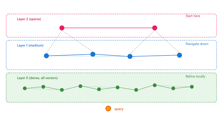
HNSW builds the graph incrementally. When a new vector is inserted, it is assigned a random maximum layer according to an exponential distribution. The algorithm then searches for the nearest neighbors of the new vector at each layer and connects them with bidirectional edges. Two parameters control the graph structure: illustrates the multi-layer graph structure of HNSW.

• M (max edges per node): Controls the graph connectivity. Higher M means more edges per node, which improves recall but increases memory usage and insertion time. Typical values range from 16 to 64.
• ef_construction (search width during build): Controls how thoroughly the algorithm searches for neighbors during insertion. Higher values produce a better graph but slow down construction. Typical values range from 100 to 400.

Figure 31.3.4: HNSW builds a multi-layer graph. Search starts at the sparse top layer and descends to the dense bottom layer for local refinement.

Search Algorithm

At query time, HNSW search begins at the top layer's entry point and greedily navigates toward the query vector. At each layer, it finds the closest node, then descends to the same node in the layer below. At the bottom layer (layer 0, which contains all vectors), it performs a more thorough local search controlled by the ef_search parameter. Higher ef_search values explore more candidates, improving recall at the cost of latency.

Algorithm: HNSW SEARCH-KNN
Input:  query q, multi-layer HNSW graph H with layers L_max .. 0,
        entry point ep at layer L_max, beam width ef, return count k
Output: top-k approximate nearest neighbors of q

  // 1. Coarse descent: greedy walk on every upper layer
  current := ep
  For lc = L_max .. 1:
      current := SEARCH-LAYER-GREEDY(q, current, layer = lc)
      // greedy means: at each step move to the neighbor closer to q;
      // stop when no neighbor improves distance(q, .)

  // 2. Beam search on the dense bottom layer (layer 0)
  W := SEARCH-LAYER-BEAM(q, current, layer = 0, ef = ef)
      // maintains a min-heap of size ef ordered by distance(q, .)
      // explores neighbors of the best frontier node until no improvement

  // 3. Truncate to k
  Return k closest elements of W (by distance to q)

SEARCH-LAYER-BEAM(q, entry, layer, ef):
  visited := {entry}
  candidates := MinHeap({entry}, key = distance(q, .))      // frontier
  W         := MaxHeap({entry}, key = distance(q, .))       // top-ef so far
  While candidates is not empty:
      c := candidates.pop_min()
      if distance(q, c) > distance(q, W.peek_max()):
          break                                             // no improvement possible
      For neighbor n in graph_layer[c]:
          if n in visited: continue
          visited.add(n)
          if distance(q, n) < distance(q, W.peek_max()) or |W| < ef:
              candidates.push(n)
              W.push(n)
              if |W| > ef: W.pop_max()
  Return W

Complexity. Query time O(log N) expected on small-world graphs; per-layer hops scale
with the local degree M (typical 16..64), so total work per query is O(ef * M * log N).

# HNSW index with FAISS
import faiss
import numpy as np
import time
dim = 768
n_vectors = 1_000_000
# Generate random normalized vectors
np.random.seed(42)
vectors = np.random.randn(n_vectors, dim).astype(np.float32)
faiss.normalize_L2(vectors)
query = np.random.randn(1, dim).astype(np.float32)
faiss.normalize_L2(query)
# Build HNSW index
# M=32: each node connected to ~32 neighbors
# ef_construction=200: search width during build
index = faiss.IndexHNSWFlat(dim, 32)
index.hnsw.efConstruction = 200
print("Building HNSW index...")
start = time.time()
index.add(vectors)
build_time = time.time() - start
print(f"Build time: {build_time:.1f}s")
print(f"Memory: ~{index.ntotal * dim * 4 / 1e9:.2f} GB (vectors only)")
# Search with different ef values to show recall/latency tradeoff
for ef_search in [16, 64, 256]:
    index.hnsw.efSearch = ef_search
    start = time.time()
    distances, indices = index.search(query, k=10)
    search_time = (time.time() - start) * 1000
    print(f"ef_search={ef_search:>3}: {search_time:.2f}ms, "
        f"top result idx={indices[0][0]}")

The layer-assignment rule that governs how often a vector lands on each layer can be written compactly as:

which produces the geometric tail $\Pr[\ell \geq k] \approx M^{-k}$. The expected number of layers therefore grows as $\log_M N$, and the greedy descent visits a constant number of nodes per layer, which is the source of the overall $O(\log N)$ query complexity.

# Build and query an HNSW index over random 384-dim vectors using hnswlib.
# Shows the two construction knobs (M, ef_construction) and the query-time
# knob (ef) that traded latency for recall in the analysis above.
import numpy as np
import hnswlib

dim = 384
num_elements = 100_000
rng = np.random.default_rng(0)
data = rng.standard_normal((num_elements, dim)).astype("float32")

# Build the graph.  M controls per-node degree; ef_construction controls the
# beam used while inserting each new point.
index = hnswlib.Index(space="cosine", dim=dim)
index.init_index(max_elements=num_elements, ef_construction=200, M=16)
index.add_items(data, np.arange(num_elements))

# Query-time accuracy/latency knob.  Higher ef = wider beam = higher recall,
# linearly higher latency.  Typical production values: ef in [50, 200].
index.set_ef(64)

query = rng.standard_normal((5, dim)).astype("float32")
ids, dists = index.knn_query(query, k=10)
print("nearest ids   :", ids[0])
print("nearest scores:", dists[0].round(3))

31.3.3 IVF: Inverted File Index

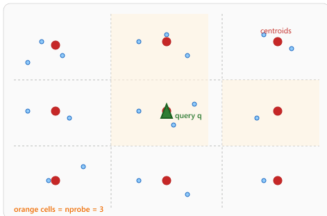
The Inverted File (IVF) index partitions the vector space into nlist regions using k-means clustering. Each vector is assigned to its nearest cluster centroid. At query time, the algorithm first identifies the nprobe closest centroids to the query, then performs an exhaustive search only within those clusters. This reduces the number of distance computations from N to approximately N × nprobe / nlist.

The expected visit count, assuming the corpus is balanced uniformly across the $k = $ nlist Voronoi cells, captures the speed knob in one line:

$$ V(n_{\text{probe}}) \;=\; n_{\text{probe}} \cdot \frac{N}{k} \;+\; k, $$

where the first term is the cost of scanning the $n_{\text{probe}}$ inverted lists touched at query time and the second term is the one-shot cost of comparing the query to every centroid. The speedup over brute force is therefore $N / V(n_{\text{probe}}) \approx k / n_{\text{probe}}$ once $N \gg k$, which is why the standard recipe sets $k \approx \sqrt{N}$ (so the two terms balance) and tunes $n_{\text{probe}}$ at query time to slide along the recall/latency curve.

Algorithm: IVF SEARCH-KNN
Input:  query q, codebook of centroids C = {c_1, .., c_nlist}, inverted lists
        I_1, .., I_nlist (each I_j holds vector IDs assigned to c_j), nprobe, k
Output: top-k approximate nearest neighbors of q

  // 1. Coarse quantization: pick the nprobe nearest centroids to q
  cand_lists := top_nprobe_argmin_j  ||q - c_j||

  // 2. Inverted-list scan: exact search within those lists only
  H := MaxHeap(size = k, key = distance)
  For j in cand_lists:
      For id in I_j:
          d := distance(q, vectors[id])
          If |H| < k or d < H.peek_max():
              H.push((id, d))
              if |H| > k: H.pop_max()
  Return H sorted ascending by d

Construction (offline):
  1. Train k-means with K = nlist centers on a sample of the corpus.
  2. For each vector v, assign it to argmin_j ||v - c_j||; append v's ID to I_j.

Cost analysis. With N vectors uniformly distributed across nlist cells:
   coarse step:   compare to nlist centroids => O(nlist * d)
   refinement:    nprobe * (N / nlist) full distances => O(nprobe * N * d / nlist)
   Total speedup over brute force: roughly nlist / nprobe
   Typical tuning: nlist = O(sqrt(N)), nprobe = 8..128 trades recall for latency.

Figure 31.3.5: IVF partitions the vector space into nlist Voronoi cells (one per centroid). At query time the algorithm scores the nprobe centroids closest to the query and exhaustively scans only the vectors inside those cells, skipping the rest of the corpus.

IVF Construction

Building an IVF index requires a training phase where k-means clustering is performed on a representative sample of the data. The number of clusters (nlist) is typically set to the square root of N, although values between 4×sqrt(N) and 16×sqrt(N) are also common. More clusters enable more selective search but require more centroids to be compared at query time.

# IVF index with FAISS
import faiss
import numpy as np
import time
dim = 768
n_vectors = 1_000_000
np.random.seed(42)
vectors = np.random.randn(n_vectors, dim).astype(np.float32)
faiss.normalize_L2(vectors)
query = np.random.randn(1, dim).astype(np.float32)
faiss.normalize_L2(query)
# IVF with flat (uncompressed) storage within each cell
nlist = 1024 # Number of Voronoi cells (clusters)
quantizer = faiss.IndexFlatIP(dim) # Inner product for normalized vectors
index = faiss.IndexIVFFlat(quantizer, dim, nlist, faiss.METRIC_INNER_PRODUCT)
# IVF requires a training step (k-means on the data)
print("Training IVF index...")
start = time.time()
index.train(vectors)
print(f"Training time: {time.time() - start:.1f}s")
# Add vectors to index
start = time.time()
index.add(vectors)
print(f"Add time: {time.time() - start:.1f}s")
# Search with different nprobe values
for nprobe in [1, 8, 32, 128]:
    index.nprobe = nprobe
    start = time.time()
    distances, indices = index.search(query, k=10)
    search_time = (time.time() - start) * 1000
    print(f"nprobe={nprobe:>3}: {search_time:.2f}ms, "
        f"searched {nprobe * n_vectors // nlist:,} vectors")

31.3.4 Tree-Based ANN: Annoy Random Projection Forests

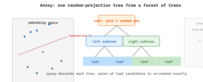
HNSW is a graph-based index and IVF is a cell-based index; the third structural family is tree-based, and the canonical implementation is Annoy (Approximate Nearest Neighbors Oh Yeah, Spotify, 2015). Annoy builds a forest of random projection trees: each tree picks two random vectors at every node, draws the perpendicular bisector between them, and recursively partitions the dataset by which side of that hyperplane each vector falls on. The leaves contain small clusters of nearby vectors. At query time the algorithm descends each tree to the leaf containing the query, unions the candidates across all trees, and re-ranks them by exact distance.

The strengths and weaknesses follow directly from the construction. The index is memory-mapped from disk (Annoy was built to serve Spotify's recommendation index without loading it into RAM), so it scales to enormous corpora on small machines. Building is embarrassingly parallel across trees because each tree is independent. Recall is tuned by adding more trees rather than by retraining, which matches a write-once-read-many catalog like a music library. The cost is that updates require rebuilding the whole index (Annoy is immutable after construction) and the per-query latency is higher than HNSW at the same recall level because the algorithm has to descend every tree. The mental map for picking among the three families: choose HNSW for low-latency in-memory search with frequent updates, IVF (often as IVFPQ) for memory-constrained billion-scale search, and Annoy for memory-mapped read-only catalogs where build simplicity and a small dependency footprint matter more than the last 10% of recall.